14.1 Introduction
Habitat loss, pollution and climate change are the primary drivers of biodiversity loss, causing ecosystems to degrade, which in turn impacts human well-being (IPBES, 2019). We depend directly on other life forms: plants are a source of food and shelter for many animals, as well as unique sources of medicine, while trees provide building materials and act as carbon sinks. Flowering plants play a vital part in supporting ecosystems, attracting pollinators that in turn enable plants to develop seeds to produce offspring (Ollerton et al., 2011). Nearly half of the world’s known wildflowers are threatened with extinction according to a new study (Bachman et al., 2024). The UK alone is reported to have lost 97% of its weed-rich meadows since the 1930s (Fuller, 1987). Wildflowers are under threat and therefore so are the pollinators they feed (Goulson et al., 2015), thus impacting directly the food that we eat (Van der Sluijs and Vaage, 2016). It is crucial to understand biodiversity trends for preservation policy planning. However, due to the amount of effort and expertise required for conventional field monitoring, there are still large gaps in our knowledge. Furthermore, ad-hoc data collection in open citizen science platforms often results in biased data because of species overrepresentation and underrepresentation (Schermer and Hogeweg, 2018).
biodiversity loss
In the last few years, deep learning – with a focus on computer vision – has been playing an essential role in large-scale automated monitoring. Recent papers (Hicks et al., 2021; Mann et al., 2022; Schouten et al., 2024) explore how object detection may be purposed for automating in-situ wildflower monitoring by identifying and counting species in images. As it turns out, wildflower monitoring combines a unique set of challenges for computer vision (Nguyen, 2016). As illustrated in Figure 14.1 these include: 1) viewpoint variations, 2) occlusion by other plants, 3) clutter, 4) light variation, 5) object deformations, as flowers are easily damaged, 6) intra-class variation, and 7) inter-class similarity. The latter two challenges are particularly hard for current models: some images of flowers in the same class may have significant visual differences, while at the same time visual similarities in shape and colour may exist between some species belonging to different classes (note that the wildflowers depicted in the last column of Figure 14.1 belong to three different species). This confusion makes it difficult even for humans to distinguish the species without deeper taxonomic expertise, and subsequently limits the performance of image-only wildflower monitoring models. Indeed, while the visual modality is rich and detailed, it lacks certain information available to human experts while doing fieldwork.
deep learning

Challenges of flower identification ‘in the wild’: 1) viewpoint variations (Papaver rhoeas); 2) occlusion (Caltha palustris); 3) clutter (Achillea millefolium); 4) light variation (Leucanthemum vulgare); 5) deformations (Bellis perennis); 6) intra-class variation (Ficaria verna); 7) inter-class similarity (Bellis perennis, Leucanthemum vulgare, Matricaria chamomilla)
Photos are crops from Eindhoven Wildflower Dataset (Schouten et al., 2024)
We therefore propose a multimodal approach that includes information on flowering phenology to help overcome the flower inter-class similarity and intra-class variation challenges for the Eindhoven Wildflower Dataset (EWD), an expert-annotated bird’s-eye view high-resolution image dataset (Schouten et al., 2024). Flowering phenology refers to the study of the timing of seasonal events in flowering plants over their growth cycle. Our approach leverages the fact that the visual characteristics as well as the presence of wildflowers at a given point in time highly depends on their estimated flowering time. In this chapter, we present a novel and large multimodal wildflower dataset and benchmark several multimodal models to encourage machine-learning research that may help us monitor, understand and ultimately preserve biodiversity.
More concretely, our contributions include:
-
A benchmark of several fusion models demonstrating that multimodal approaches significantly outperform image-only methods.
-
An open multimodal dataset for wildflower monitoring, uniquely combining high-quality annotated wildflower images from the Netherlands (Schouten et al., 2024) with flowering phenology measurements from a public database (NDFF, n.d.).
multimodal approach
Eindhoven Wildflower Dataset (EWD)
The remainder of this paper is structured as follows. Section 14.2 discusses prior work in automated flower monitoring. Section 14.3 discusses some object detection and multimodality preliminaries, while section 14.4 defines, in formal language, the task of identifying and counting wildflowers using multimodal data. Section 14.5 details how the dataset was created. Section 14.6 describes the methodology and section 14.7 presents the benchmarks and the results. Section 14.8 discusses current limitations and section 14.9 concludes.
14.2 Flower recognition with computer vision
Wildflowers are intensely studied in biodiversity research since their clear visual characteristics, such as colour, shape and texture, enable large-scale monitoring (Tran et al., 2018). Earlier methods to automatically identify wildflowers involve explicit coding of morphological features (colour, texture, shape) using handcrafted image processing filters (Wäldchen and Mäder, 2015; Hong and Choi, 2012), but since the introduction of Convolutional Neural Network (CNN) architectures (He et al., 2016; Krizhevsky et al., 2012; Simonyan and Zisserman, 2014; Szegedy et al., 2016), wildflower identification has mostly transitioned to deep learning. However, training a CNN with sufficient generalization capabilities to solve this task requires a large, labelled dataset with significant intra-class diversity. The PlantCLEF challenge (Krishna et al., 2020) targets the identification of plants (including flowers) with computer vision methods, holding over two million images of about 80,000 species. Another large-scale citizen science database for flower identification is iNaturalist (iNaturalist, n.d.), comprising over 65 million images of about 140,000 species. In these settings, however, usually a close-up of a single flower (or inflorescence) located at the centre of the image has been captured, rather than a wider image of a natural scene containing many wildflowers at the same time.
coding of morphological features
Recently, wildflower monitoring use cases have been introduced that deploy object detection to identify multiple flowers in an image, using bounding boxes (BBs) to annotate the images. Remote sensing data has also been used for a variety of downstream tasks such as detecting visiting pollinators on flowers (Tran et al., 2018), detecting the blooming stages of a species (Ärje et al., 2019), and measuring flower phenology (Mann et al., 2022). However, in these studies, there are no visually similar species within the data.
using bounding boxes (BBs)
Other studies use datasets with a larger variety of species which do have inter-class similarity: the Oxford102 (Nilsback and Zisserman, 2008) and Jenna30 (Seeland et al., 2017) datasets comprise both single and multiple flower instances in an image, annotated to investigate flower detection and classification for 102 and 30 species, respectively (Patel and Patel, 2020). Wildflower monitoring to estimate nectar sugar mass was done using images of 25 species in weed-rich grasslands in the UK (Hicks et al., 2021), and flower detection from different image perspectives (entire flower, frontal, and lateral view) have been done for 10 species (Abbas et al., 2022). Although not publicly available, drone-based image acquisition datasets have been collected in mountainous areas for 25 species in Switzerland (Gallmann et al., 2022). In these studies, however, data and annotation quality varies wildly. For real-world images with many visually similar species, precisely labelled and annotated high-quality images are essential (Elphick, 2008; Farnsworth et al., 2013). EWD offers a significantly larger collection of wildflower images comprising 160 species from various habitats in the Netherlands, with guaranteed in-situ high-quality expert-annotated images based on well-established annotation guidelines (Schouten et al., 2024).
14.3 Object detection and multimodality preliminaries
Over the course of just a few years, deep learning has gained immense popularity. We briefly review the field of object detection within deep learning and its state-of-the-art model Faster R-CNN (Faster Region-based Convolutional Network) before discussing multimodal learning related work.
14.3.1 Object detection
Object detection is often confused with image recognition, the fundamental computer vision task. Figure 14.2 shows an example of the distinction between image recognition and object detection. Image recognition assigns one label to an entire image. A picture of a flower receives the label ‘flower’; a picture of three flowers also receives the label ‘flower’. Object detection, on the other hand, draws a BB around each object and labels each individual box. The model predicts where each object is and what label should be applied. In that way, object detection provides more information about an image than whole-image labelling, i.e. through its unique ability to locate objects within an image. Identifying the right object is still a classification task, localizing an object can be expressed as a regression task. A common approach to predicting a BB around an object is to predict the coordinates of the object’s centre (i.e. horizontal and vertical coordinates within the image) and height and width of the BB box; thus, four continuous numbers.
Image recognition and object detection comparison. Image recognition (first and third) labels the entire image, while object detection (second and fourth) localizes objects in an image by drawing bounding boxes around them and then labels them accordingly. Photos are crops from EWD images (Schouten et al., 2024)
Photos are crops from Eindhoven Wildflower Dataset (Schouten et al., 2024)
The major drawback of object detection, however, is the cost of annotating. To annotate objects’ BBs and labels for each image in a dataset is still the hardest and most time-consuming part of object detection. However, if the labels and BBs have been obtained for every object in an image, then an object detection model can be trained. Notable object detection models include Faster R-CNN (Ren, 2016), YOLO (You Only Look Once) (Redmon, 2016), or SSD (Single Shot Detector) (Liu et al., 2016). Note that object detection is essential for many real-world tasks such as diagnosis (recognizing deficiencies), monitoring (counting objects in an image) and navigation (recognizing various objects in a scene and acting upon that information).
14.3.2 Faster R-CNN
Most of the current state-of-the-art object detection models are built on the groundwork laid by the Faster R-CNN model. A Faster R-CNN model has several stages, as shown in Figure 14.3. An entire image and a set of object BBs with corresponding labels is passed as input. First, the image passes through the backbone dense convolutional neural network (CNN). Digital images consist of a series of numbers, arranged in a 3-layered 2D array (one layer for ‘red’, one layer for ‘green’, and one layer for ‘blue’). This is how a computer perceives an image, and CNNs build on this idea. The idea is that, given an array of numbers, the network is able to use low-level features such as edges and curves to generate abstract high-level features in the later convolutional layers. After passing through several convolutional and pooling layers (that basically perform filter operations and downsample), a feature map is generated. The feature map is a spatially dense tensor that represents the learned features of the image.
convolutional neural network (CNN)
Diagram of the Faster R-CNN architecture
Using the feature map and the image’s annotated bounding boxes, the Region Proposal Network (RPN) predicts whether there is an object or not and the bounding box of those objects. Initially, RPN generates anchor points at regular intervals over the image, which will act as a prior to predict object proposals. Predefined anchor boxes of different sizes and aspect ratios are placed at the centre of each anchor point. The network refines these anchor boxes throughout training to better match actual object positions and sizes. A basic geometrical concept for evaluating how well an object detection model predicts BBs is the Intersection over Union (IoU). This concept measures the area overlap between the predicted BB and the annotated or target BB, divided by the area of their union. An IoU close to the maximum value of 1 is considered very good, whereas values close to 0 mean both bounding boxes nearly do not intercept each other. For each anchor, the RPN predicts two set of parameters, namely the probability of the anchor containing an object (also known as an objectness score) and adjustments to the anchor boxes’ coordinates to match the actual object’s shape (four scores, one for each box corner).
Region Proposal Network (RPN)
Intersection over Union (IoU)
The region proposals are of different sizes, so a technique called Region of Interest (ROI) pooling is used to resize them before passing them through the Faster R-CNN network. The network flattens the proposed region feature map into a fully connected layer and learns to label categories using the cross-entropy loss and ground truth boxes using the least square errors (L2) regression loss. The cross-entropy loss (or log loss) measures the performance of a classification model whose output is a probability value between 0 and 1. The L2 regression loss minimizes the error, which is the sum of all the squared differences between the true value and the predicted value.
Region of Interest (ROI)
14.3.3 Evaluation metrics explained
Object detection models are therefore more complex since they combine both location prediction and object classification. So, what happens if the model detects the correct class but at the wrong location? One approach is to define an IoU threshold. The object detection evaluation metrics need to know what a ‘correct detection’ and an ‘incorrect detection’ are. By setting an IoU threshold, the user can classify a detection as correct or incorrect. For example, we may consider that a prediction is correct only if the IoU is greater than a threshold of 0.5 and the predicted class is correct. The evaluation metrics can then be more or less restrictive as thresholds closer to 1 require almost perfect detections, whereas a threshold near 0 accepts even poor detections.
The standard metrics used in the object detection tasks are the mean average precision (mAP) and mean average recall (mAR). These metrics are derived from the confusion matrix by counting correct and wrong classifications, according to the chosen IoU threshold (see Figure 14.9 for an example). Each detected BB belongs to one of the four components of the confusion matrix and is classified per class observation:
-
True Positive (TP): a correct detection of the observed ground truth class.
-
False Positive (FP): an incorrect detection of another class or background.
-
False Negative (FN): an undetected bounding box of the observed ground truth class.
-
True Negative (TN): a correct detection of no class/background (no bounding box placed).
mean average precision (mAP)
mean average recall (mAR)
Precision measures the accuracy of positive predictions, i.e. TP/(TP+FP), while recall measures the ratio of positive predictions that are correctly detected by the classifier, i.e. TP/(TP+FN). Precision and recall values range from 0 (lowest value) to 1 (best value). Ideally, both precision and recall should be high. The trade-off between precision and recall can be visualized in a so-called Precision-Recall (PR) curve.
Average precision (AP) shows the model’s performance by taking the area under the PR curve and computing the average precision at different recall values (i.e. 0, 0.1, …,1) for a given IoU threshold. In multi-class object detection (i.e. there are more than two classes), the AP is computed for each class and then the mAP is computed. The mAR is computed similarly, except that for average recall (AR) we average recall values over several IoU thresholds (i.e. [0.5, 0.95] with a 0.05 step), then compute mAR in multi-class object detection.
14.3.4 Data fusion and multimodality
Current computer vision research that is beyond state of the art involves multimodal input data. Modalities can be divided into four main groups (Pawłowski et al., 2023):
-
Tabular data: observations are stored as rows and their features as columns.
-
Graphs: observations are vertices, and their features are in the form of edges between individual vertices.
-
Signals: observations are files of appropriate extension (images:.jpeg, audio:.wav, etc.) and their features are the numerical data provided within files.
-
Sequences: observations are in the form of characters/words/documents, where the type of character/word corresponds to features.
Data fusion strategies – combining several of these modalities – can be categorised as early fusion and late fusion (Huang et al., 2020).1 The schemas of early and late fusion are depicted in Figure 14.4. Early fusion, also denoted as data-level or feature-level fusion, simply joins data or features into common feature space, usually by concatenation. Late fusion, or decision-level fusion, joins prediction results from unimodal models (such as probability logits or categorical outcomes in classification tasks) to achieve multimodal prediction. In this study, we focus on early feature-level fusion techniques as they usually surpass the unimodal counterparts of late fusion and offer more flexibility in the AI-pipeline (Cui et al., 2023; Stahlschmidt et al., 2022).
data fusion strategies
Data fusion techniques: (left) early fusion, and (right) late fusion
In this study, we only leverage from one non-image modality. The common practice is to perform simple operations of concatenation, element-wise summation or element-wise multiplication, with the last two operations requiring feature vectors of different modalities to be converted into the same shape. It is difficult to compare the performance of different operation-based feature-level fusions, since different studies were done on different data with different settings. However, in general multimodal solutions significantly outperform solutions using a single modality, but it might yield inferior performance when learning complex interactions of different modalities.
Most multimodality studies are done in the domain of medical image analysis. To give some examples: Holste et al. (2021) compare these operation-based methods joining medical imaging with non-image data medical records for breast cancer classification. They extend the ResNet50 (He et al., 2016) architecture with early fusion strategies. Their multimodal models outperform the unimodal model, with the early fusion strategy achieving superior performance. Chen et al. (2019) propose a multimodal architecture which is based on Faster R-CNN for cervical cancer classification. While they also fuse features from two types of medical images, they fuse non-image features extracted from clinical tests with learned image features by using one fully connected layer.
14.4 Task definition
Figure 14.5 provides an overview of the learning task we aim to solve. First, the flowering phenology is a graphical representation of the timing and duration of seasonal flowering for a species, with time (e.g. days, weeks, months) on the horizontal axis and a phenology estimate on the vertical axis (Haggerty and Mazer, 2008). Given a set of images, each with a creation date d, and a set of possible species s₁, …, sn that we aim to detect, we extract the flowering phenology estimates for that point in time: 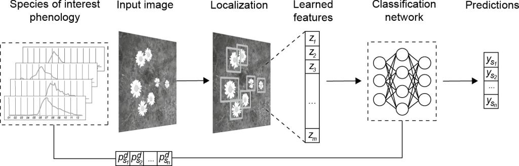 . We then aim to train a model m that, for each detected flower in the image, receives the (pre-trained) image features z₁, …, zm and flowering phenology estimates
  as input, and predicts the vector y = (ys1, ..., ysn) of probabilities for each possible species.
An overview of our multimodal object detection solution
We aim to use annotated images and flowering phenology estimates in conjunction to classify species; thus, our task can be considered a supervised multimodal object detection problem. We use a pre-trained object detection architecture for image feature extraction and localization and attempt early feature fusion by concatenating non-image data (i.e. tabular data  ) within the Faster R-CNN architecture. Our goal during training is to reduce misclassifications of visually similar species.
14.5 Dataset
Our dataset is constructed using data from two open data resources: wildflower images from the Eindhoven Wildflower Dataset (EWD) (Schouten et al., 2024), an expert-annotated high-resolution image dataset, and flowering phenology estimates from the Dutch National Database Flora and Fauna (NDFF, n.d.). Both datasets are from the Netherlands. To the best of our knowledge, it is the first multimodal dataset allowing fine-grained differentiation of a set of visually similar wildflowers using phenology. Similar approaches consider spatio-temporal location data (Mac Aodha et al., 2019; De Lutio et al., 2021). However, their temporal information is limited by the presence-only data, which inherently lacks information about species growth cycle.
14.5.1 Image dataset
We fully leverage the image and annotation quality of EWD, which contains top-view flowering plant images with expert-annotated BBs around individual flowers. The images were collected in-situ from flower beds of approximately 1 m² taken (near-)vertically downwards at a height ranging from 1.5 to 1.9 m, in the region of Eindhoven, the Netherlands, over the years 2021 and 2022. Annotations are formatted in Pascal VOC (Visual Object Classes), containing BBs with their corresponding species labels stored in a human readable XML format. There are over 65,000 annotations for 160 species with a long-tailed species distribution.
Since the EWD images are significantly large (6720 × 4480 pixels) and today’s most advanced Faster R-CNN architectures have a maximum input size that is significantly lower (1,333 pixels on either axis) (Li et al., 2021), we slice the original images into 15 (5 × 3) tiles. Tiles without object annotations are disregarded. We employ a cutting approach that is aware of the presence of annotations in the image and attempts to find the least damaging way to cut it. A helper function is employed to divide the input images into slices that approximate the target size. Figure 14.6 shows an example of image sliced into 15 tiles with this heuristic approach. We train, validate and test models with image tiles in our experiments.
An example of an EWD image sliced into tiles, taken from Schouten et al. (2024). The dashed lines show equally sized tiles. Note the difference in the number of cut wildflowers (Calty palustris in this case) between the two tiling schemes
14.5.2 Flower phenology data
We collect flowering phenology data from NDFF (NDFF, n.d.). Flowering phenology is a graphical representation of the timing and duration of blooming for a particular flowering plant over a specific period (Haggerty and Mazer, 2008). The data is modelled based on observations from the period 2000–2021. Observations are collected by volunteers and professionals and validated by experts. Only approved observations (over 2 million in total!) are included. Observation counts from each year are converted into a circular format and then averaged. The peak and median are then calculated from the averaged circular density data, as well as the day numbers on which 10%, 20%, 80% and 90% of the observations are made. A box plot is then generated from this data for each species. The flowering phenology is therefore determined on the basis of a percentile value (Van der Hak, 2022).
14.5.3 Data alignment
The phenology data is aligned with the image data based on the exact time that the image was taken, as described in section 14.4. To analyse whether the phenology data matches the wildflowers in the images, we selected two groups of common wildflowers; each group contains three species with high inter-class similarity. Figure 14.7 shows a sample of the selected species, while Table 14.1 describes the details of the two groups.
Selected flower species grouped by visual similarity. Group 1: Buttercup (aggregate), Caltha palustris, Ficaria verna; Group 2: Bellis perennis, Chamomile (aggregate), Leucanthemum vulgare. Photos are crops randomly sampled from EWD
Selected flower species dataset description. Subspecies visually indistinguishable in the field are merged in the EWD dataset: Ranunculus acris and Ranunculus repens are labelled as Buttercup (aggregate), while Matricaria chamomilla and Matricaria maritima are labelled as Chamomile (aggregate)
Figure 14.8 shows an overview of the flowering phenology (top) and histograms of the distributions by day of the year (bottom) for each species in each group. All species are denoted by their botanical name. Species in Group 1 belong to the Ranunculaceae family with yellow flowers in blooming stage, while species in Group 2 belong to the Asteraceae family with flowerheads (white radial flowers and yellow disc flowers in the centre) in blooming stage. We can indeed observe different peaks for each species. The merged species labelled Buttercup (aggregate) have statistically similar flowering phenology estimates. Matricaria chamomilla and Matricaria maritima have different estimates, with the latter recurring all year round. We select the Matricaria chamomilla flowering phenology estimates for the merged species Chamomile (aggregate). Species objects are counted from 2021 and 2022 images per day. More images of Buttercup (aggregate) and Chamomile (aggregate) have been collected in a single day. The observations and flowering phenology peaks correlate in Group 1. In Group 2 there is more overlap for observations and flowering phenology peaks.
Data alignment overview for both groups: (top) flowering phenology estimates from NDFF for the selected species and (bottom) histogram of objects counts from EWD for the selected species. The horizontal axis is the day of year ranging from 1 to 365, while the vertical axis is (top) the phenological index, normalized from 0 to 1, and (bottom) an object count
14.5.4 Dataset splits
To avoid bias, we randomly selected images such that the total object amount matches that of the training-validation-test sets over all species. In object detection, a single image can contain observations of multiple objects as well as different types of objects, making it challenging to create a balanced dataset. If an image is selected because it contains a specific wildflower, it may also include other wildflowers incidentally. By providing the sample sizes for the training, validation and test sets, theoretically all permutations that achieve the exact desired numbers can be computed. However, this approach becomes exponentially time-consuming as the dataset grows larger. To address this issue, we use a trial-and-error approach, making numerous attempts and stopping early when a solution is found. With this approach, we randomly select images amounting to 550 objects for the training sets, 100 objects for validation set, and 50 objects in test set for each selected species.
14.6 Methodology
14.6.1 Models
14.6.1.1 Baselines
In line with the existing literature on flower monitoring (Gallmann et al., 2022; Hicks et al., 2021; Schouten et al., 2024), we propose using the Faster R-CNN object detection model as our main image-only baseline. We compare this with other state-of-the-art object detection models such as SSD and YOLOv8. Furthermore, we test the vision capabilities of the state-of-the-art Multimodal Large Language Model (MLLM) with vision (GPT-4v) (OpenAI, n.d.) and LLaVA-1.5 (Liu et al., 2023), which we do not fine-tune. We also investigate the classification performance from just the phenology features with XGBoost classifier (Chen and Guestrin, 2016), as well as from just image classification, using ResNet-50 (He et al., 2016).
Faster R-CNN object detection model
Multimodal Large Language Model (MLLM)
14.6.1.2 Feature fusion
We proposed feature-level fusion combining features from images and flowering phenology into a single high-dimensional feature vector using concatenation (Cui, et al., 2023). To this end, we extended the Faster R-CNN architecture. Faster R-CNN works by first extracting feature vectors from a backbone CNN, after which the RPN (Region Proposal Network) generated region proposals in the image and a fixed-length feature vector for each region, which was in turn fed into successive fully connected layers, followed by two outputs: the species classification head and the BB location regression head. The classifier produced probability values of each proposed object belonging to n categories and one catch-all background category. The regressor head output four offsets (x, y, h, w) from the RPN more precisely, where (x, y) specified the values of the position of the left corner, and (h, w) the height and width of the window. The flowering phenology was passed into a 1-dimensional vector of length n in the classifier. The values of the flowering phenology feature vector were extracted from the flowering phenology graphs at a given image creation date and passed as input alongside the image. We concatenated feature vectors from each Faster R-CNN proposed region with the flowering phenology vector before feeding it to the classifier. During training, we computed the classification loss using cross-entropy. We used the image features from generated proposals for the BB regressor.
14.6.1.3 Learned feature fusion model
We also proposed to simultaneously learn features from flowering phenology, then combined them with the image features. Although simple and effective, feature concatenation might not exploit the complex correlation between the heterogeneous modalities (Cui et al., 2023). We used the flower phenology 1-dimensional vector of length n categories to learn a vector of the same length as the image features, which we then combined. Thus, we processed the low-dimensional flowering phenology features by fully connected layers to the same dimension of image features before fusion. To understand how different fusion operations impacted predictive performance, we experimented with three fusion operations: 1) concatenation, 2) element-wise multiplication and 3) element-wise addition (Holste et al., 2021).
14.6.2 Experimental setup
We trained separate models for each group for 30 epochs. We used five seeds for training-validation-test sets. Each experiment was run on training-validation-test sets from each seed and results reported the average. We only inferred the test set on the MLLMs. Training, validation and test sets followed the splitting described in Section 14.5. For the Faster R-CNN models the image features are learned with ResNet-50 (He et al., 2016) with pre-trained weights, which performed best in wildflower detection studies (Patel and Patel, 2020; Schouten et al., 2024). We used the open-source PyTorch framework and the Faster-RCNN (Ren, 2016) and SSD (Liu et al., 2016) model, as provided in the TorchVision library. We used the Ultralytics framework for the YOLOv8 model. We leveraged the OpenAI API to utilize GPT-4v, the vision-enabled variant of the GPT-4 model and OllamaChat integrated with LLaVA v1.5, for the advanced image processing and analysis task. The Faster R-CNN classifier ResNet50 was fine-tuned for the image-only classification. Finally, for the phenology-only classification, we leveraged from the XGBoost library.
14.6.3 Metrics
We measured object detection performance using COCO metrics (Lin et al., 2015), i.e. we reported the AP per class and the mAP over all classes at 0.50 and [0.50,0.95] interval with 0.05 step IoU threshold (see also Section 14.3.3). We also reported the coefficient matrix with confidence threshold over 0.75 and IoU threshold over 0.50. We reported the precision scores for the classification models after training. All scores were averaged over the five seeds. In addition, we used the non-parametric paired sample t-test to determine whether the different values across performance scores from each seed were statistically significant (at a significance level of 0.05) or occurred by chance.
14.7 Results
Table 14.2 offers a holistic view of each model performance. We observe that fusion models outperform image-only models for both groups. This highlights the value of flowering phenology for our task. Precision increases significantly with additional features for the learned feature fusion with elementwise concatenation and addition variants (p < 0.1). The learned feature fusion method likely captures more nuanced relationships between learned features from both modalities and optimizes the combination process, leading to improved performance compared to a simple concatenation approach. The variant using element-wise addition fusion had the best predictive performance, which could imply that the learned image and flowering phenology features were relevant and complementary.
Table 14.3 shows the AP scores per class for statistically different fusion models. Buttercup (aggregate) and Chamomile (aggregate) species have significantly higher AP scores in the learned feature fusion variants, which may indicate that there are significantly fewer missed detections and/or misclassifications. However, these scores describe the performance of object detection models based on both the accuracy of object localization and the ability to detect all instances of objects, and do not directly capture misclassifications. To better evaluate misclassification, Figure 14.9 shows the performance scores for each species in a confusion matrix averaged over five runs. We report baseline and elementwise addition learned feature fusion variant at confidence score over 0.75 and IoU threshold over 0.50. Interestingly, there are fewer missed detections in the fusion model at a 0.75 confidence. This may indicate that more robust and generalizable features are learned with the addition of flowering phenology. There are also significantly fewer misclassifications in Group 1. There are slightly more misclassifications between Bellis perennis and Leucanthemum vulgare in the multimodal variant. This is primarily caused by the training-validation-test splits which did not take into account image creation date distribution. There are more Bellis perennis image samples at the flowering phenology peak of Leucanthemum vulgare. In Group 1, data distribution for each species matches flowering phenology peaks, hence the significant class differentiation. Thus, we suggest balancing training, validation and test set splits also on dates.
Test results on Group 1 and Group 2 for all models averaged over five seeds. Best results are shown in bold
Test results per species class for the image-only baseline and the best performing feature fusion models averaged over five seeds
We also experimented with MLLMs, but we found lower performance for the task of object detection, as shown in Table 14.4. Recent inclusion of vision in MLLMs shows great potential indeed. However, the wildflower detection use case is still challenging for these models. While the largest MLLM, GPT-4v, can now identify and provide information about objects within images, it is still limited in object detection functionality. According to the OpenAI guide on GPT-4v, the model may give approximate counts for objects in images. After conducting some tests on GPT-4v, we found that the GPT-4v API and the GPT-4v web app version returned coordinates when given a direct prompt, but the coordinates were not correct. In both versions, just requesting counts worked better. However, when feeding the full resolution (6720 × 4480 pixels) EWD images, the model hallucinated. When feeding image tiles the counts were better approximated, but not for all images. We tested with the test datasets from each group. The current behaviour therefore shows that the model is capable of object detection but does not perform well. Recent approaches use the ‘classic’ computer vision model in tandem with GPT-4v as an object detection model. Thus, GPT-4v alone in its current state is not near object detection state of the art.
Open-source LLaVA is less efficient than GPT-4v as an object detection model. Similar to GPT-4v, when asked to generate the bounding box coordinates, the model seemed to hallucinate. Furthermore, the model is reluctant to give counts when flowers are cluttered and smaller. The model LLaVA also fails to correctly identify the visually similar species, which was expected as LlaVA is smaller than GPT-4v. However, unlike GPT-4v, the model can be fine-tuned. Ultimately, LLaVA is limited by hallucinations and weak in-depth reasoning common to many LMMs.
Test results on Group 1 and Group 2 for all classification models averaged over five seeds, hence average precision (AP)
Confusion matrix with confidence threshold over 0.75 and IoU threshold over 0.50 for image-only and learned feature-level fusion elementwise addition models
We also report the classification performance on the selected species. We used the same train-validation-test splits and trained two classifiers, using images only and phenology only. ResNet50 was trained on 30 epochs. We also inferred state-of-the-art MLLMs on the test set. We feed the box images, not the entire image, to the classifiers and MLLMs. The classifier using phenology always predicts the correct class. Training an image classifier is also more efficient with higher performance scores. Object detection models are evaluated using metrics like mean mAP, which consider both classification accuracy and localization. These metrics are more stringent than those used for classification alone (such as accuracy or precision-recall), and as a result, they tend to reflect lower precision scores.
14.8 Limitations
Firstly, flowering phenology estimates do not take into account recent rapid climate change trends, modelling an average of all observations over the last 21 years. In our study we use image data from 2021 and 2022. Generally, climate change will advance the timing of seasonal events for the majority of flowering plants, which is already well documented (Geissler et al., 2023). The flowering phenology estimates could perhaps be improved based on annual weather measurements for a better representation of the species encounter. Furthermore, reliable flowering phenology estimates may not be publicly available for species worldwide. Nonetheless, monthly flower counts from citizen science platforms – like iNaturalist or the Dutch platform waarneming.nl – may be used to compute flowering phenology estimates similarly (Van der Hak, 2022). Subsequently, the image dataset has imbalanced sample dates. This is a limitation shared with other datasets, and a common issue in in-situ data collection.
Furthermore, the dataset may not include sufficient images with different backgrounds, lighting conditions, and object poses. Data augmenting techniques such as random flipping, addition of noise, blur, contrast and brightness shifts can be leveraged to improve the robustness of the models (Rebuffi et al., 2021). Another limitation of our study might be the small training setup. However, training with more image data may not always improve model performance (Zhu et al., 2011). Nevertheless, the results of the multimodal models are still remarkable. Finally, the limited amount of annotated data currently available for object detection purposes related to wildflowers still proves to be a significant obstacle in current computer vision research.
14.9 Conclusion
We propose a multimodal dataset and benchmark for wildflower monitoring using their flowering phenology estimates. The multimodal dataset includes high-quality annotated wildflower images and flowering phenology estimates from the Netherlands. We detail the process of collecting and using the flowering phenology estimates. We also present results for the dataset on a range of data fusion variants. Extensive experiments have corroborated the effectiveness of our multimodal approach in reducing misclassification. We are planning a next version of the dataset that will include flowering phenology that accounts for changes in climate over time. As this work is intended to directly impact wildflower monitoring, we hope such input will be valuable to researchers seeking to understand biodiversity and climate change, as well as policymakers interested in evaluating preservation priorities across different areas of land.
References
Abbas, T., Razzaq, A., Zia, M.A., Mumtaz, I., Saleem, M.A., Akbar, W., … and Shivachi, C.S., 2022. Deep neural networks for automatic flower species localization and recognition. Computational intelligence and neuroscience, 2022:9359353.
Ärje, J., Milioris, D., Tran, D.T., Jepsen, J.U., Raitoharju, J., Gabbouj, M., … and Høye, T.T., 2019. Automatic flower detection and classification system using a light-weight convolutional neural network. In: EUSIPCO Workshop on Signal Processing, Computer Vision and Deep Learning for Autonomous Systems.
Bachman, S.P., Brown, M.J., Leão, T.C., Nic Lughadha, E. and Walker, B.E., 2024. Extinction risk predictions for the world’s flowering plants to support their conservation. New phytologist, 242:797–808.
Chen, T. and Guestrin, C., 2016. Xgboost: A scalable tree boosting system. In: Proceedings of the 22nd ACM SIGKDD international conference on knowledge discovery and data mining, pp. 785–794.
Chen, T., Ma, X., Ying, X., Wang, W., Yuan, C., Lu, W., … and Wu, J., 2019. Multi-modal fusion learning for cervical dysplasia diagnosis. In: IEEE 16th international symposium on biomedical imaging (ISBI 2019), pp. 1505–1509.
Cui, C., Yang, H., Wang, Y., Zhao, S., Asad, Z., Coburn, L.A., … and Huo, Y., 2023. Deep multimodal fusion of image and non-image data in disease diagnosis and prognosis: a review. Progress in biomedical engineering, 5:022001.
De Lutio, R., She, Y., D’Aronco, S., Russo, S., Brun, P., Wegner, J.D. and Schindler, K., 2021. Digital taxonomist: identifying plant species in community scientists’ photographs. ISPRS journal of photogrammetry and remote sensing, 182:112–121.
Elphick, C.S., 2008. How you count counts: the importance of methods research in applied ecology. Journal of applied ecology, 45:1313–1320.
Farnsworth, E.J., Chu, M., Kress, W.J., Neill, A.K., Best, J.H., Pickering, J., … and Ellison, A.M., 2013. Next-generation field guides. BioScience, 63:891–899.
Fuller, R. 1987. The changing extent and conservation interest of lowland grasslands in England and Wales: a review of grassland surveys 1930–1984. Biological conservation, 40:281–300.
Gallmann, J., Schüpbach, B., Jacot, K., Albrecht, M., Winizki, J., Kirchgessner, N. and Aasen, H., 2022. Flower mapping in grasslands with drones and deep learning. Frontiers in plant science, 12:774965.
Geissler, C., Davidson, A. and Niesenbaum, R.A., 2023. The influence of climate warming on flowering phenology in relation to historical annual and seasonal temperatures and plant functional traits. PeerJ, 11, e15188.
Goulson, D. Nicholls, E., Botías, C., and Rotheray, E.L., 2015. Bee declines driven by combined stress from parasites, pesticides, and lack of flowers. Science, 347:1255957.
Haggerty, B.P. and Mazer, S.J., 2008. The phenology handbook. University of California, Santa Barbara, P41.
He, K., Zhang, X., Ren, S. and Sun, J., 2016. Deep residual learning for image recognition. In: Proceedings of the IEEE conference on computer vision and pattern recognition, pp. 770–778.
Hicks, D., Baude, M., Kratz, C., Ouvrard, P. and Stone, G., 2021. Deep learning object detection to estimate the nectar sugar mass of flowering vegetation. Ecological solutions and evidence, 2:e12099.
Holste, G., Partridge, S.C., Rahbar, H., Biswas, D., Lee, C.I. and Alessio, A.M., 2021. End- to-end learning of fused image and non-image features for improved breast cancer classification from MRI. In: Proceedings of the IEEE/CVF International Conference on Computer Vision, pp. 3294–3303.
Hong, S.W. and Choi, L., 2012. Automatic recognition of flowers through color and edge-based contour detection. In: 3rd International conference on image processing theory, tools and applications (IPTA), pp. 141–146.
Huang, S.C., Pareek, A., Zamanian, R., Banerjee, I., and Lungren, M.P., 2020. Multimodal fusion with deep neural networks for leveraging CT imaging and electronic health record: a case-study in pulmonary embolism detection. Scientific reports, 10:22147.
iNaturalist (n.d.). iNaturalist. Retrieved April, 2024 from https://www.inaturalist.org/taxa/47125-Angiospermae.
IPBES (2019). Global assessment report on biodiversity and ecosystem services of the Intergovernmental Science-Policy Platform on Biodiversity and Ecosystem Services.
Krishna, N.H., Rakesh, M. and Ram Kaushik R., 2020. Plant species identification using transfer learning-PlantCLEF 2020. In: CLEF (Working Notes).
Krizhevsky, A., Sutskever, I. and Hinton, G.E., 2012. Imagenet classification with deep convolutional neural networks. Advances in neural information processing systems, 25.
Lin, T.Y., Maire, M., Belongie, S., Hays, J., Perona, P., Ramanan, D., … and Zitnick, C.L., 2014. Microsoft COCO: common objects in context. In: Computer vision – ECCV 2014: 13th European Conference, Zurich, Switzerland, September 6–12, 2014, Proceedings, Part V 13. Springer International Publishing, pp. 740–755.
Liu, W., Anguelov, D., Erhan, D., Szegedy, C., Reed, S., Fu, C.Y. and Berg, A.C., 2016. SSD: single shot multibox detector. In: Computer vision – ECCV 2016: 14th European Conference, Amsterdam, The Netherlands, October 11–14, 2016, Proceedings, Part I 14. Springer International Publishing, pp. 21–37.
Liu, H., Li, C., Wu, Q. and Lee, Y.J., 2024. Visual instruction tuning. Advances in neural information processing systems, 36.
Mac Aodha, O., Cole, E. and Perona, P., 2019. Presence-only geographical priors for fine- grained image classification. In: Proceedings of the IEEE/CVF International Conference on Computer Vision, pp. 9596–9606.
Mann, H.M., Iosifidis, A., Jepsen, J.U., Welker, J.M., Loonen, M.J. and Høye, T.T., 2022. Automatic flower detection and phenology monitoring using time‐lapse cameras and deep learning. Remote sensing in ecology and conservation, 8:765–777.
NDFF (n.d.). NDFF distribution atlas. Retrieved April, 2024 from https://www.verspreidingsatlas.nl.
Nguyen, T.T.N., Le, V.T., Le, T.L., Hai, V., Pantuwong, N. and Yagi, Y., 2016. Flower species identification using deep convolutional neural networks. In: AUN/SEED-Net Regional Conference for Computer and Information Engineering.
Nilsback, M.E. and Zisserman, A., 2008. Automated flower classification over a large number of classes. In: 6th Indian conference on computer vision, graphics & image processing, pp. 722–729.
Ollerton, J., Winfree, R. and Tarrant, S., 2011. How many flowering plants are pollinated by animals? Oikos, 120:321–326.
OpenAI, n.d. GPT-4 with vision capabilities. Retrieved June, 2024 from https://openai.com.
Patel, I. and Patel, S., 2020. An optimized deep learning model for flower classification using NAS-FPN and faster R-CNN. International journal of scientific & technology research, 9:5308–5318.
Pawłowski, M., Wróblewska, A. and Sysko-Romańczuk, S., 2023. Effective techniques for multimodal data fusion: a comparative analysis. Sensors, 23:2381.
Rebuffi, S.A., Gowal, S., Calian, D.A., Stimberg, F., Wiles, O. and Mann, T.A., 2021. Data augmentation can improve robustness. Advances in neural information processing systems, 34:29935–29948.
Redmon, J., 2016. You only look once: unified, real-time object detection. In: Proceedings of the IEEE conference on computer vision and pattern recognition.
Ren, S., 2015. Faster R-CNN: towards real-time object detection with region proposal networks. arXiv preprint arXiv:1506.01497.
Schermer, M. and Hogeweg, L., 2018. Supporting citizen scientists with automatic species identification using deep learning image recognition models. Biodiversity information science and standards.
Schouten, G., Michielsen, B.S.H.T. and Gravendeel, B., 2024. Data-centric AI approach for automated wildflower monitoring. PLoS One, 19:e0302958.
Seeland, M., Rzanny, M., Alaqraa, N., Wäldchen, J. and Mäder, P., 2017. Plant species classification using flower images – a comparative study of local feature representations. PLoS One, 12:e0170629.
Simonyan, K. and Zisserman, A., 2014. Very deep convolutional networks for large-scale image recognition. arXiv preprint arXiv:1409.1556.
Stahlschmidt, S.R., Ulfenborg, B. and Synnergren, J., 2022. Multimodal deep learning for biomedical data fusion: a review. Briefings in Bioinformatics, 23:bbab569.
Szegedy, C., Vanhoucke, V., Ioffe, S., Shlens, J. and Wojna, Z., 2016. Rethinking the inception architecture for computer vision. In: Proceedings of the IEEE conference on computer vision and pattern recognition, pp. 2818–2826.
Tran, D.T., Høye, T.T., Gabbouj, M. and Iosifidis, A., 2018. Automatic flower and visitor detection system. In: 26th European Signal Processing Conference (Eusipco) (pp. 405–409).
Van der Hak, D.D., 2022. Phenology diagram generator. Retrieved May, 2024 from https://github.com/Desharin/phenology_diagram_generator.
Van der Sluijs, J.P. and Vaage, N.S., 2016. Pollinators and global food security: the need for holistic global stewardship. Food ethics, 1:75–91.
Wäldchen, J. and Mäder, P., 2018. Plant species identification using computer vision techniques: a systematic literature review. Archives of computational methods in engineering, 25:507–543.
Zhu, X., Vondrick, C., Ramanan, D. and Fowlkes, C.C., 2012. Do we need more training data or better models for object detection? In: BMVC, 3.
Huang et al. (2020) also discern intermediate fusion. This is in essence similar to early fusion, but instead of just joining original data features, it learns high-dimensional features (typically through a neural network) before joining them into the common feature space.