Abstract
This article shows how standard econometric methods, such as Ordinary Least Squares (OLS), provide a valuable basis for understanding state-of-the-art Machine Learning. We introduce nonlinearity within a polynomial regression framework to illustrate the biasâvariance trade-off and overfitting and then extend the discussion to regularization methods such as LASSO. The model-selection procedure, i.e., cross-validation, is broken down into manageable steps, each illustrated with visual aids, to clarify how Supervised Machine Learning predicts outcomes. Subsequent sections explain the limitations of these prediction methods and how they can be adapted for causal inference. We also highlight the potential and limitations of Machine Learning in variable selection for regression models to increase the replicability and credibility of empirical results and thus contribute to the p-value debate.
1. Introduction
Machine Learning (ML) predicts outcomes by selecting from a large set of candidate models, thus serving as a dimension-reduction tool. This is vital for agricultural and applied economists, who face complex modeling choices that critically shape policy evaluations. Deepening the understanding of how ML algorithms operate helps researchers and practitioners to evaluate the strengths and limitations of these methods. Much of the necessary background is already taught in standard econometrics and statistics courses. The aim of this guide is to provide a practical overview of how those familiar concepts underpin modern ML methods.
Several excellent reviews address ML in agricultural and applied economics (Athey and Imbens, 2019; Storm et al., 2020). These surveys provide detailed and accessible overviews of ML techniques and demonstrate how they can enhance the toolkit available to applied researchers. Against this background, the main contributions of this guide are twofold:
(1) We bridge the gap between examples that intuitively explain variable selection using a classical regression framework and regularization methods such as the Least Absolute Shrinkage and Selection Operator (LASSO).
(2) We review the expected outcome model to highlight one of the major limitations of standard ML techniques for causal inference. We then demonstrate how ML can be adapted to overcome this limitation using double variable selection and double ML.
Although ML adds a data-driven approach to model selection, it does not replace careful theoretical reasoning. The p-value debate, for example, has underscored the need for students and applied researchers to critically reflect on their methodological choices (Heckelei et al., 2023). Therefore, we not only aim to clarify how ML predicts outcomes and is adapted for causal inference, but also discuss issues such as pâvalue mining and how ML can help to increase replicability and credibility of empirical results.
This guide provides a step-by-step introduction to the model selection process, with particular emphasis on what the âlearningâ in ML entails. A key focus is on how Supervised ML can facilitate variable selection (Belloni et al., 2014a,b; Urminsky et al., 2016). On the one hand, variable selection is a secondary problem in classical laboratory experiments, where observation units are randomly assigned to a treatment group, or in field experiments, where real natural events are interpreted as randomized experiments (Paluck and Green, 2009). On the other hand, if the treatment is not randomly assigned, confounding factors may bias inferences about treatment effects. In such cases, a multiple regression analysis can be deployed in which confounders are included as covariates in the model.
Regression models are also often fitted to nonexperimental data because they allow âwhat natural scientists are able to do in a controlled laboratory setting: keep other factors fixedâ (Wooldridge, 2015: p. 77). Here, variation in social and political variables may produce certain forms of random assignment that mimic a true experiment (Dunning, 2010). A major challenge is to make statistical adjustments to eliminate bias in comparisons between treated and control groups. However, even without causal claims, regression analysis can be used to determine the joint distribution and associated parameters of the variables of interest (Holland, 1986).
Researchers may pursue a variety of objectives and analytical strategies in different contexts, but these may come at a cost in terms of the credibility, simplicity, and transparency of the empirical techniques used (Dunning, 2010). For example, there is concern that many empirical findings in the scientific literature are false and cannot be replicated (Ioannidis, 2005). One factor contributing to this problem could be the treatment of model and variable selection and the subsequent inference (Berk et al., 2013; Leamer, 1983). Given the complexities of model selection and estimation, establishing universal guidelines is challenging. However, if certain techniques contribute to low replicability, it is crucial to define what makes a âgoodâ model, not merely in terms of a single measure, but in relation to the broader context in which empirical outcomes are derived and presented. This paper explores how ML can serve as a valuable tool for model selection within this context.
This paper emphasizes the importance of understanding ML fundamentals, particularly cross-validation (i.e., the âlearningâ in ML), by breaking these concepts down into small, manageable steps. We employ simulations, examples, and visual aids to illustrate how ML algorithms operate in principle. The paper demonstrates how standard econometric principles and techniques, such as Ordinary Least Squares (OLS), provide an excellent foundation for grasping state-of-the-art ML techniques.
Section 2 presents model complexity via nonlinearities, using bivariate polynomial regressions. Section 3 introduces a statistical model and illustrates the variance-bias tradeâoff and overfitting in prediction. These concepts are demonstrated step by step using graphical examples of Leave-One-Out-Cross-Validation (LOOCV). Section 4 expands to shrinkage estimators, showing how methods like LASSO perform variable selection for prediction. Section 5 reviews the expected outcome model and illustrates omitted variable bias arising from ML variable selection. A Monte Carlo experiment replicates one of the key insights in Belloni et al. (2014a,b). Section 6 shows how ML variable selection is adapted for causal inference (Belloni et al., 2014a,b). The section also addresses pâvalue mining and replicability, highlighting potential and limitations to help practitioners and students make more robust variableâselection decisions (Urminsky et al., 2016). Section 7 generalizes from double variable selection to double ML and highlights its connection to the FrischâWaughâLovell theorem. This section also illustrates how modern ML methods, such as random forests and deep neural nets, can be used for causal inference (Chernozhukov et al., 2018). Section 8 concludes and offers further reading.
2. Model complexity and model fit
We start this section similarly to the introduction in Athey and Imbens (2019), beginning with the perspective of Breiman (2001), who distinguishes two cultures in statistical modeling. One culture assumes that the data are generated by a statistical model, while the other focuses on the data and largely neglects the underlying statistical model. In the spirit of the latter, this section disregards the statistical model. This approach emphasizes that our primary interest at this stage is not in estimating parameters that determine the joint or conditional distribution of a variable of interest. Rather, our goal is to find a model that simply fits the data.
We are looking for a vector of inputs, Xâ² = (X1, X2, â¦, Xp), that correlates with a vector of outcomes, Y. The link function estimated from the data is denoted by  , where p represents the model complexity. We introduce model complexity through the lens of nonlinearities. As a leading example in this paper, we rely on bivariate regression, where model complexity is introduced by incorporating polynomial terms of the input variable:

Citation: International Food and Agribusiness Management Review 28, 2 (2025) ; 10.22434/ifamr.1087
Adding polynomials adds non-linearities, which can be seen from the first derivative of this function:
Citation: International Food and Agribusiness Management Review 28, 2 (2025) ; 10.22434/ifamr.1087
In the linear case (â
p = 1) the first derivative  , i.e., the change in the outcome, is constant for any given input level. In contrast, for p = 2, the derivate is
  , i.e., the change in the outcome depends on the level of the input via
  .
.
Given some representative sample observations, {xi1, ⦠xip, yi}, we can define the sum of squared distances between the regression line and the actual datapoints:
Citation: International Food and Agribusiness Management Review 28, 2 (2025) ; 10.22434/ifamr.1087
Minimizing the Residual Sum of Squares (RSSp) using Ordinary Least Squares (OLS) is a fundamental concept in econometrics and forms the cornerstone of most textbooks. While the core idea remains the same, its treatment may vary depending on the mathematical tools employed (e.g., Mittelhammer, 2013: p. 434; Pesaran, 2015: p. 4). Based on the OLS estimation, we can define the variance decomposition as (e.g., Pesaran, 2015: p. 8):
Citation: International Food and Agribusiness Management Review 28, 2 (2025) ; 10.22434/ifamr.1087
The term TSS measures the Total Sum of Squared deviations of the outcome variable from its mean, yÌ. This measure of variation can be decomposed into the Explained Sum of Squares, which increases if the input variable correlates with the outcome variable and the Sum of Squared Residual term. Averaging the second term gives the mean squared error:
Citation: International Food and Agribusiness Management Review 28, 2 (2025) ; 10.22434/ifamr.1087
We can also calculate another measure of goodness of fit, which quantifies the proportion of variation in the outcome variable that is explained by the model:
Citation: International Food and Agribusiness Management Review 28, 2 (2025) ; 10.22434/ifamr.1087
The MSEp is therefore inversely related to the R2. In general, adding more input variables to a model cannot decrease the R2. Put it differently, increasing model complexity p, will decrease MSEp, a point that becomes crucial when discussing overfitting. In the next section, we present a numerical illustration showing how increasing model complexity affects MSEp.
2.1 Illustration
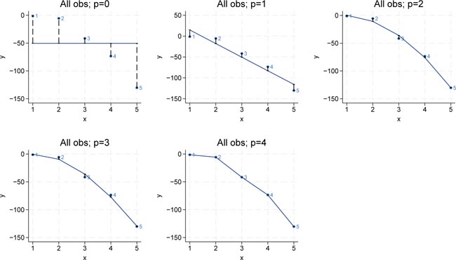
We use five simulated data points for our illustration. In the next section, we elaborate on the source of these data points. By adding enough polynomial terms of a single input variable, one can achieve a perfect fit to any outcome variable. Figure 1 shows scatter plots of polynomial regressions with degrees p = 1â4.
MSE and model complexity. Bivariate polynomial regressions with five observations (n = 5) and p = 1â4. Source: Own representation based on simulated datapoints using StataCorp (2023).
Citation: International Food and Agribusiness Management Review 28, 2 (2025) ; 10.22434/ifamr.1087
When the model complexity is p = 1 (a linear model), the first derivative is simply , which means that the change in Y is constant for any given value of X. In contrast, for a quadratic model (â
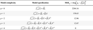
p = 2), the first derivative is indicating that the change in Y depends on the level of X; that is, the effect of X on Y is no longer constant but varies with the level of X. Adding more polynomial terms increases the degree of nonlinearity. In the extreme, if enough polynomial terms are added, the model can fit the observed outcome perfectly. Correspondingly, increasing the model complexity leads to a better in-sample fit and a decrease in the MSE, as demonstrated in Table 1.
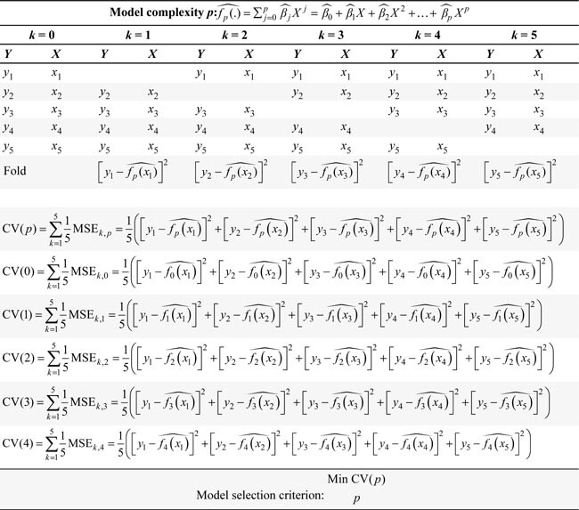
Model complexity and MSE
Citation: International Food and Agribusiness Management Review 28, 2 (2025) ; 10.22434/ifamr.1087
The main task discussed next is to select variables that fit the data points while recognizing that some of the observed variation is random. To understand this, we introduce the concept of a statistical model, a formal framework that represents both the systematic component and the random noise in the data.
3. The statistical model and model selection
Holland (1986) defines the standard statistical model as one that relates variables over a population, from which the joint distribution and associational parameters can be derived. This framework is especially useful when the goal is to understand the underlying process generating the data rather than to enumerate every possible observation. Such an approach enables us to generalize findings beyond the dataset at hand, which we treat as a sample. Hereafter, we refer to the basic statistical model, in which the outcome Y is defined as
Y = fp(Xâ
) +
The term fp(Xâ
) links the input X to the output Y, while
In the infinite population approach, randomness is introduced through the error term, that is, each observation is considered a random draw from a probability distribution (e.g., Dumelle et al., 2022; Fisher, 1922: pp. 311â312; Sterba, 2009). In many model-based regression frameworks, we can then condition on the values of the input variables, treating them as fixed, which leaves the outcome variable random.
This contrasts with the design-based perspective, where randomness comes from the sampling procedure itself, that is, we imagine that each data point is a random draw from a finite population (e.g., Dumelle et al., 2022; Neyman, 1934: pp. 567â570; Sterba, 2009). In this framework, the population is considered a fixed, finite collection of individuals or objects. In some cases, data may be available for every member of the population, or the sample may effectively represent the entire population.
The primary purpose of introducing a statistical model here is to account for randomness in our analysis. By incorporating randomness, we acknowledge that an idiosyncratic component is inherent in the actual dataset we observe, meaning that a perfect fit of the data is not only unattainable but also undesirable. If we do achieve a perfect fit, it may indicate that we have overfitted the model. This concept is the basis of the subsequent simulations. The advantage of simulations, compared to real-world datasets, is that we know the exact properties of the data.
Depending on the statistical framework, we can view  be a potential polynomial estimator for the link function of the statistical model fp(Xâ
). Then the expected MSE of the estimator is defined as,
be a potential polynomial estimator for the link function of the statistical model fp(Xâ
). Then the expected MSE of the estimator is defined as,
Citation: International Food and Agribusiness Management Review 28, 2 (2025) ; 10.22434/ifamr.1087
and these expressions can be further rearranged:1
Citation: International Food and Agribusiness Management Review 28, 2 (2025) ; 10.22434/ifamr.1087
On the one hand, if the model underfits because an overly restrictive functional form is chosen, it will not capture all the reducible variation in the data. Prediction is biased. Typically, as the flexibility of the functional form increases, the bias decreases, but variance increases. Overfitting means that the estimated functional form is too complex and/or some noise in the data has been fitted.
At its core, the power of ML lies in its ability to automatically select a model that balances the variance-bias trade-off in prediction. As Hawkins (2004) notes: âA model overfits if it is more complex than another model that fits equally well. This means that recognizing overfitting involves not only the comparison of the simpler and the more complex model but also the issue of how you measure the fit of a model.â One approach is to use information criteria such as AIC and BIC (Akaike, 1973; Schwarz, 1978). These criteria impose a penalty based on degrees of freedom, so that when two models fit equally well, the simpler one is preferred. Another powerful method is cross-validation (e.g., Golub et al., 1979; Shao, 1993; Stone, 1977).
The fundamental building block of cross-validation is a sample split. The first sample is called the training data, denoted as  , where n represents the number of observations. The MSE over Tr is given by:
Citation: International Food and Agribusiness Management Review 28, 2 (2025) ; 10.22434/ifamr.1087
Minimizing MSETr,p over all possible models is likely to result in overly complex and overfitted models. Instead, we introduce a separate dataset that has not been used in model training, the test data, denoted as  . The measure of fit based on the test data is defined as
Citation: International Food and Agribusiness Management Review 28, 2 (2025) ; 10.22434/ifamr.1087
It is crucial that the test dataset remains separate from the training data. A decrease in MSETe,p indicates improved predictive power and greater generalizability of the model.
Next, we define cross-validation, a technique designed to use the training data as efficiently as possible during model selection. The process begins by dividing the training set into K folds. The k-th fold (k = 1, ⦠Kâ
) serves as the validation set, while the remaining data are used for training. When training the p-th model (â
p = 1, â¦, P), we obtain  , i.e., the model fit derived from the training data with the k-th fold removed. We can compute the MSE for the k-th fold:
Citation: International Food and Agribusiness Management Review 28, 2 (2025) ; 10.22434/ifamr.1087
where i â Fk. Finally, to obtain the cross-validation estimate of the prediction error, we compute the average over all folds,
Citation: International Food and Agribusiness Management Review 28, 2 (2025) ; 10.22434/ifamr.1087
where nk are the number of observations in the k-th fold. Cross-validation reshuffles the dataset by repeatedly splitting and reassembling it K times, effectively mimicking a resampling procedure. This approach enhances efficiency by generating K variations of the original training dataset, enabling the evaluation of multiple model specifications. These variations provide context on how the best model specification compares to other alternatives. As a result, K-fold cross-validation can also play a role in sensitivity analysis (see Dudoit and Van der Laan, 2005; Robins et al., 2007).
Choosing a highly restrictive functional form results in a model with low variance but high bias, leading to a high in-sample MSETr,p. Such a model will also perform poorly out-of-sample, resulting in a high MSETe,p. Conversely, an overfitted model achieves a low in-sample MSETr,p because the model captures even the noise in the training data. However, the model will perform poorly on the test sample i.e. a high MSETe,p since the fitted noise does not generalize to new data.
Next, we show how to determine the polynomial order. Understanding how cross-validation works clarifies how LASSO performs feature selection and, by extension, how Supervised ML algorithms operate.
3.1 Illustration
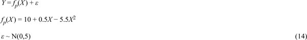
We proceed with the same five data points from the previous illustration. The five observations were drawn from the following statistical model:
Citation: International Food and Agribusiness Management Review 28, 2 (2025) ; 10.22434/ifamr.1087
Note, in most non-experimental cases we do not know the statistical model. Given the framework of polynomial regressions, our task in model selection is to find the model with the optimal complexity, in our case, a quadratic model (â p = 2). We fit polynomial models of increasing order and perform Leave-One-Out-Cross-Validation (LOOCV) for each model. In the LOOCV setup, each fold contains only one observation (i.e., nk = 1), the total number of observations is n = 5, and the number of folds is K = 5 (Hastie et al., 2009, p. 242). Table 2 displays the LOOCV for each model complexity (â p = 1â4).
Model complexity and LOOCV model selection
Citation: International Food and Agribusiness Management Review 28, 2 (2025) ; 10.22434/ifamr.1087
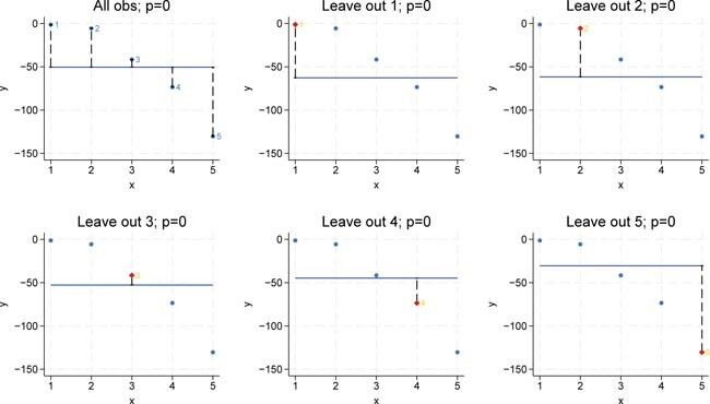
For each fold, we run a regression leaving the k-th observation out. We then use the resulting model to predict the outcome for the left-out observation and calculate the squared residual. Repeating this procedure for k = 1â5 mimics a resampling process in which each observation is left out once, allowing us to assess how the model predicts the unused data point. Finally, we average the five squared prediction errors to obtain the cross-validation error for each model complexity.
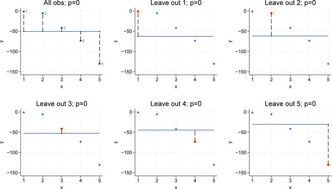
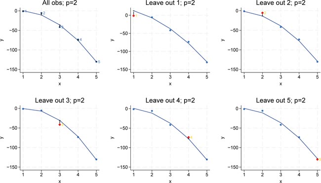
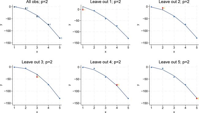
Figure 2 illustrates a regression using the full sample with complexity p = 0, i.e., a model containing only one constant term, as well as five additional regressions where each plot omits one observation. In each leave-one-out scenario, the omitted observation is predicted. The left-out observation is highlighted in red, and its distance to the constant regression line is then squared. Averaging these squared distances across all folds yields the overall leave-one-out error.
LOOCV for p = 0. Bivariate polynomial regressions with five observations (n = 5), LOOCV and p = 0. Source: Own representation based on simulated datapoints using StataCorp (2023).
Citation: International Food and Agribusiness Management Review 28, 2 (2025) ; 10.22434/ifamr.1087
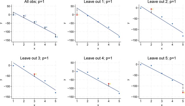
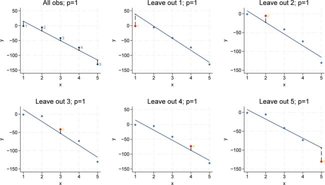
LOOCV for p = 1. Bivariate polynomial regressions with five observations (n = 5), LOOCV and p = 1. Source: Own representation based on simulated datapoints using StataCorp (2023).
Citation: International Food and Agribusiness Management Review 28, 2 (2025) ; 10.22434/ifamr.1087
LOOCV for p = 2. Bivariate polynomial regressions with five observations (n = 5), LOOCV and p = 2. Source: Own representation based on simulated datapoints using StataCorp (2023).
Citation: International Food and Agribusiness Management Review 28, 2 (2025) ; 10.22434/ifamr.1087
The next set of graphs applies the same procedure for model complexity p = 1, i.e., the linear model, to illustrate how a first-degree polynomial (a straight line) fits the data under the leave-one-out approach. Again, each regression minimizes the squared distance based on the training sample, i.e., it minimizes the training MSE. The leftâout observation is marked in red and is not used in fitting the model, it is used to calculate the outâofâsample MSE. Note that each time a different observation is omitted, the training data change slightly, leading to a different fit.
In the quadratic model (complexity p = 2), the outâofâsample MSE is even smaller than in the linear case. This indicates that when we add the quadratic term to our model, the predictions for the leftâout observations are improved. In other words, the model with p = 2 appears to capture the underlying data structure better, resulting in lower out-of-sample prediction errors. Figure 4 shows the case for p = 2, corresponding to a quadratic model.
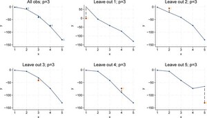
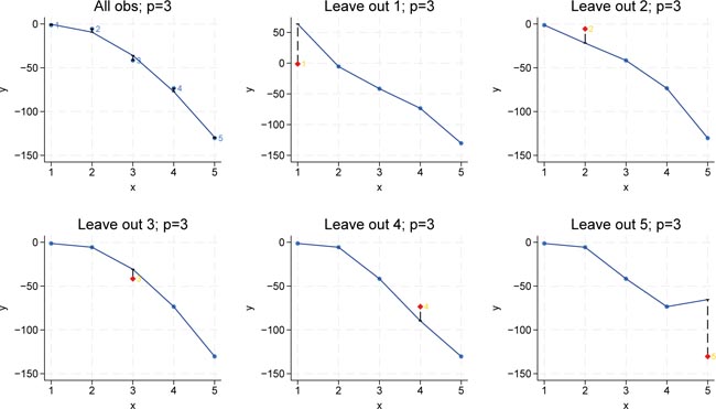
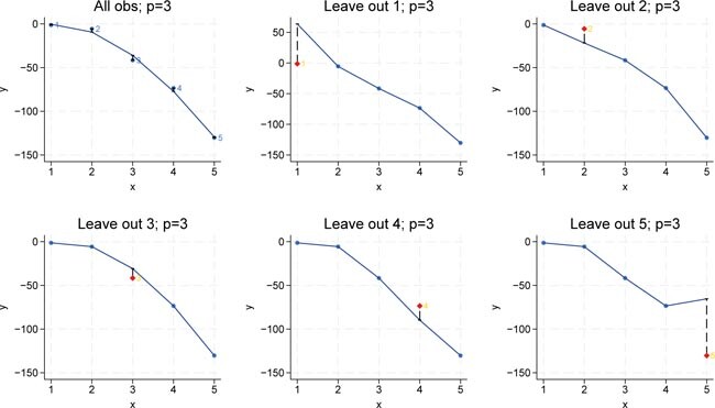
However, it is important to keep in mind that increasing model complexity beyond a certain point may eventually lead to overfitting, where the in-sample error continues to decrease while the outâofâsample error starts to increase. Figure 5 shows the cubic model (complexity p = 2). The full-sample regression produces a low MSE because the model fits the observed data nearly perfectly. However, when we compute the leave-one-out MSE, which represents the out-of-sample prediction error, we observe that the error is considerably larger. This discrepancy indicates overfitting: the model has fitted the idiosyncratic part of the sample data and its out-of-sample-performance suffers. Put it differently, even though the in-sample MSE is small for p = 3, the out-of-sample error reveals that the model does not generalize to new datapoints.
LOOCV for p = 3. Bivariate polynomial regressions with five observations (n = 5), LOOCV and p = 3. Source: Own representation based on simulated datapoints using StataCorp (2023).
Citation: International Food and Agribusiness Management Review 28, 2 (2025) ; 10.22434/ifamr.1087
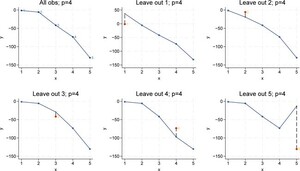
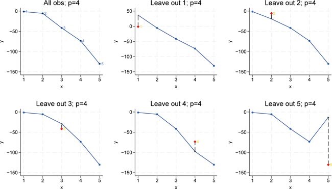
In the model with four polynomials of the input variable (â p = 4), the full-sample regression achieves a perfect fit on the observed data, with the in-sample MSE equal to zero. However, when we calculate the leave-one-out MSE, we observe that the prediction error is even larger than that of the cubic model. This pattern reinforces the overfitting phenomenon: although increasing the complexity to p = 4 allows the model to perfectly capture the training data (resulting in zero in-sample error), it fails to generalize, as evidenced by the increased out-of-sample error. Figure 6 shows the results for p = 4.
LOOCV for p = 4. Bivariate polynomial regressions with five observations (n = 5), LOOCV and p = 4. Source: Own representation based on simulated datapoints using StataCorp (2023).
Citation: International Food and Agribusiness Management Review 28, 2 (2025) ; 10.22434/ifamr.1087
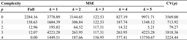
Table 3 summarizes the results for the models of increasing complexity. In this table, the following measures are reported for each model complexity p. The MSE is calculated using the entire sample (i.e., the in-sample error). The squared errors for each of the five leave-one-out folds follow (i.e., the out-of-sample error for each omitted observation). The last row is the average of the five CV errors, representing the overall cross-validated MSE.
Model selection and MSE
Citation: International Food and Agribusiness Management Review 28, 2 (2025) ; 10.22434/ifamr.1087
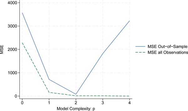
Table 3 shows that model complexity increases from p = 0 (only a constant) to p = 4 (a quartic model). The in-sample (full-fitted) MSE steadily decreases. In contrast, the out-of-sample MSE (CV) initially decreases (indicating improved prediction) but then increases for the more complex models, reflecting the overfitting phenomenon where the model fits the training data perfectly but performs poorly on new data. This illustrates the bias-variance trade-off in model selection. If we minimize the MSE using the full sample, we tend to choose a model with maximum complexity (â p = 4) because the model will fit not only the systematic pattern in the data but also the random noise. In contrast, if we minimize the MSE based on out-of-sample prediction (using cross-validation), we choose a lower complexity (â p = 2). This occurs because the statistical model includes an idiosyncratic, random component; fitting that noise too closely actually degrades predictive performance when the model is applied to new data. Figure 7 shows that while the full-sample MSE continues to decrease with increasing model complexity, the out-of-sample prediction error reaches a minimum at a lower complexity level (â p = 2).
Cross-validation function and model complexity. MSE of Bivariate Polynomial Regressions with five observations (n = 5), LOOCV and p = 0â4. Source: Own representation based on simulated datapoints using StataCorp (2023).
Citation: International Food and Agribusiness Management Review 28, 2 (2025) ; 10.22434/ifamr.1087
In summary, selecting the model based on minimizing the prediction error in the test sample means looking for input combinations that correlate with the outcome. The function CV(â p) provides a test error curve over different model complexities and we pick the functional form that minimizes the test error.
4. Variable selection and LASSO
We start this section with the optimization problem of the OLS estimator. The goal is to choose model parameters to minimize the target function, i.e., the RSS:
Citation: International Food and Agribusiness Management Review 28, 2 (2025) ; 10.22434/ifamr.1087
Alternatively, we can consider a shrinkage estimator. The fundamental insight into how the estimator works can be traced back to Steinâs paradox: when estimating three or more parameters simultaneously, it is possible to achieve a lower expected MSE than if the parameters were considered separately (Efron and Morris, 1977). Equation (16) shows the optimization problem of the shrinkage estimator:
Citation: International Food and Agribusiness Management Review 28, 2 (2025) ; 10.22434/ifamr.1087
Compared to equation (15), there is an additional term. From a modelâselection perspective, this is a penalty term. From a Bayesian perspective, the term can be interpreted as a prior on the model parameters. In Bayesian inference, the posterior distribution is derived by combining the likelihood of the data with a prior distribution that may reflect pre-existing beliefs about the parameters before observing the data (Gelman et al., 2013: p. 20). The parameter
From a modelâselection perspective, the parameter
The term |.|r represents a norm. When r = 0, the penalty simply counts the number of parameters, meaning model complexity is measured by how many variables are included. For r = 1, the estimator is known as the LASSO, where some coefficients may be shrunk exactly to zero. In contrast, with r = 2, the estimator is a ridge regression, where all coefficients are shrunk toward zero but not eliminated.
The ridge regression is useful to discuss in this context because it can be easily shown to extend standard OLS estimation. A ridge regression can be interpreted as biased estimator in the context of the Gauss-Markov theorem (Pesaran, 2015: pp. 34â38 and 259â262). Furthermore, as the penalty increases, the bias increases while the variance decreases, embodying the bias-variance trade-off. For further discussions on MSE, variance and bias in the context of ridge regression, see Farebrother (1976), Theobald (1974) and Taboga (2021).
An important feature of the LASSO is that model selection also entails variable selection, because some coefficients can be reduced to zero.2 Choosing a smaller set of inputs from a larger pool is a dimension reduction. Applying LASSO requires the computation of many different models. The algorithm orders models by
In the subsequent section, we illustrate the link between the polynomial regressions and LASSO. Previously, we determined the optimal polynomial order sequentially. Now, we provide the polynomial terms as inputs to LASSO and let it perform feature selection. Thus, model complexity is controlled by
4.1 Illustration
As in the previous section, we use the same five data points generated from the statistical model in equation (14). To mirror the polynomial regression framework, we include the terms X, Xâ
2, Xâ
3, Xâ
4 as inputs. In the previous example, we compared exactly five models, one for each polynomial order. LASSO, by contrast, considers many subsets of {X, Xâ
2, Xâ
3, Xâ
4} as
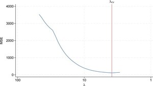
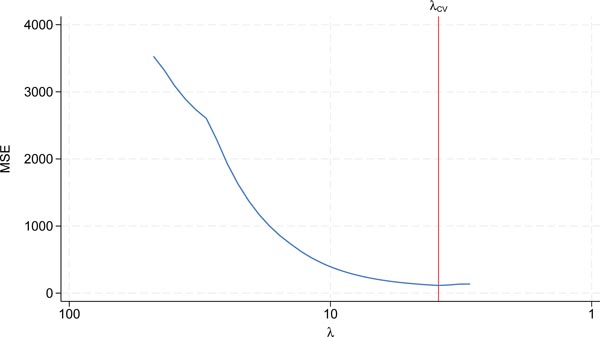
We again perform LOOCV for each model. We run the model leaving out the k-th observation, predicting the outcome for that leftâout observation, and calculate the squared residual. Repeating this for all folds and averaging gives the CV error for a given model complexity, governed by
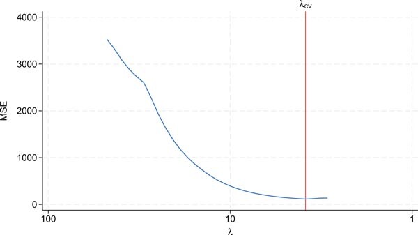
Cross-validation function for LASSO. The MSE of the cross-validation function for LOOCV with five observations (n = 5) is plotted in blue. λ CV = 39 is the cross-validation minimum plotted in red. The number of inputs selected is two. Source: Own representation based on simulated datapoints using StataCorp (2023).
Citation: International Food and Agribusiness Management Review 28, 2 (2025) ; 10.22434/ifamr.1087
The optimal shrinkage intensity is
Further, although
In real-world applications, with many data points and many potential inputs, the number of possible models grows rapidly. Thus, it is also important to consider trade-offs between predictive accuracy, model parsimony, and computational efficiency.
Choosing the model with the lowest outâofâsample MSE effectively balances the bias-variance trade-off. While this is beneficial for prediction, it poses challenges for causal inference, where estimating the partial effect of an input requires careful control for unmeasured confounders. To understand this, we introduce the expected outcome model in the next section.
5. The expected outcome model and omitted variable bias
As Rubin (1990) noted, many causal inference concepts emerged from agricultural experiments that used controlled, randomized trials to assess treatment effects, such as fertilizer, crop varieties, or irrigation on yields. These early studies laid the groundwork for formalizing causal effects as comparisons between potential outcomes under different treatments. For example, the potential outcomes framework has its roots in randomized experiments as in Neyman (1923).
The potential outcome model provides a language for researchers to explicitly state and examine their causal assumptions.3 In a randomized trial, each unit is assumed to have a set of potential outcomes (one for each treatment), even though only one is observed. Random assignment ensures that any differences in outcomes are attributable to the treatments rather than confounding factors, forming the basis for modern causal inference methods. To understand the core concepts, we examine the expected outcome model and its relation to standard regression as outlined in the fundamental reference Angrist and Pischke (2009).
We will concentrate on getting to the regression formulation as quickly as possible and start with the idea of a classical laboratory experiment, where observation units are randomly assigned to a treatment group. The variable D may be such a treatment, which is randomly assigned. The observed outcomes Y is distinguished by the potential outcome Y1 if D = 1 and the potential outcome Y0 if D = 0:
Citation: International Food and Agribusiness Management Review 28, 2 (2025) ; 10.22434/ifamr.1087
This formulation highlights the crucial distinction between the pair of potential outcomes (Y1, Y0) and the realized outcome Y. Specifically, if an individual is treated, then Y1 is observed while Y0 serves as the counterfactual outcome. Conversely, if an individual is not treated, Y0 is observed and Y1 becomes the counterfactual. This is a fundamental insight: to determine the effectiveness of a treatment, we must compare a measurable outcome with an outcome that, by definition, cannot be observed. Allowing for some randomness in the untreated outcome, denoted as u, we obtain (Angrist and Pischke, 2009, p. 22):
Y =
This allows us to represent the constant average treatment effect within a linear regression framework:
One of the key assumptions in causal inference is unconfoundedness. Unconfoundedness posits that the treatment assignment is as good as random. If the treatment is not randomly assigned, confounding factors bias inferences about treatment effects. One way to address this problem is to use matching techniques to reduce the bias introduced by confounders (Rosenbaum and Rubin, 1983). To show the implications for the regression framework, we assume that we can measure the relevant confounding factors using observed control variables. If the treatment assignment is not random, there is additional variation in the error term,
u = fâ
(Xâ
) +
where fâ
(Xâ
) is the link function of the additional inputs and
Y =
Finally, we assume that the functional form of the control variables can be approximated by a linear mode, i.e.,  :
:
Citation: International Food and Agribusiness Management Review 28, 2 (2025) ; 10.22434/ifamr.1087
It is important to emphasize that unconfoundedness (a concept from the expected outcome model) and strong exogeneity (in regression analysis) are not identical, but they are closely related (Imbens and Wooldridge, 2009). We do not want to delve too deeply into causal concepts at this point. The key argument is that if random assignment is violated, sample selection bias arises, which can be represented in a regression framework with the omitted variable bias formular (Angrist and Pischke; 2009: Chapter 2). For p = 1, omitting variable X results in the following bias:
Citation: International Food and Agribusiness Management Review 28, 2 (2025) ; 10.22434/ifamr.1087
We assume here that X is the only omitted variable. If the omitted variable is correlated with other included inputs, the bias will be more complex than what this formula suggests (see Wooldridge, 2015: pp. 88â91, for the standard omitted variable bias).
Although there are many threats to the validity of causal inference such as the inclusion of âbad controlsâ (Hünermund et al., 2023) among other issues, the problem of omitted variable bias is especially important in the context of ML. ML variable selection tends to lead, on average, to omitted variable bias (Belloni, Chernozhukov and Hansen, 2014a,b). In other words, if we repeatedly apply a ML procedure (such as LASSO) on different samples and then use the selected variables to run a regression, the resulting regression coefficients cannot be interpreted as partial effects on average (i.e., as the treatment effect, holding all else constant). In the next subsection, we illustrate the omitted variable bias using a simulation.
5.1 Illustration
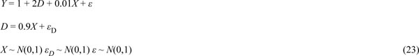
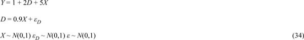
We conduct a Monte Carlo experiment. We simulate 1000 observations from the model below:
Citation: International Food and Agribusiness Management Review 28, 2 (2025) ; 10.22434/ifamr.1087
The first line in equation (23) states that the outcome correlates with the control variable and the treatment. The constant does not impact the results. The second line introduces a correlation between the treatment variable and the control. For illustration the control variable is strongly correlated with the treatment, yet its direct effect in the regression is kept small. However, experimenting with the relationship between the control and the treatment, adjusting the influence of the control on the outcome, and adding more inputs can be very useful to explore how changes in these relationships affect model estimates and to better understand the robustness of the results.
The variable D is continuous in this example, and we are interested in the partial effect of D on Y. Although D has been introduced as binary in the expected outcome model to keep the notation and interpretation of the average treatment effect (treated versus untreated) simple, in practice many treatments vary in intensity. In addition, Belloni et al. (2014a,b) also use a continuous treatment variable in their simulation study.
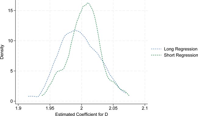
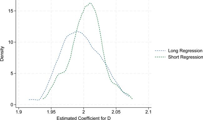
The simulation is repeated 100 times. For each we run the regression of Y on D and X. This is the long regression. We also run a regression based on LASSO feature selection. Finally, a kernel density estimator is applied to illustrate the distribution of the estimated coefficient for D, which is plotted in Figure 9.
Monte Carlo simulation for single LASSO feature selection. Each replication consists of 1000 simulated observations. The blue dashed line represents the kernel estimate of the 100 estimations of the long regression model. The green dashed line represents the kernel estimate of the 100 short regression estimations. Source: Own representation based on simulated datapoints using StataCorp (2023).
Citation: International Food and Agribusiness Management Review 28, 2 (2025) ; 10.22434/ifamr.1087
As shown in the graph, the OLS estimates in blue (âLong Regressionâ) differ on average from the estimates based on LASSO selection in green (âShort Regressionâ). The reason is that LASSO omits the variable X on average, resulting in the short regression as previously described. Consequently, the systematic difference between the two sets of estimates can be interpreted as omitted variable bias introduced by LASSO feature selection.
6. Double variable selection and omitted variable bias
If adequately trained, LASSO and other ML algorithms are efficient at predicting out-of-sample. A variable that is highly correlated with other included variables tends to add little predictive power, which is why LASSO is likely to drop such a variable. While this variable may be unimportant for prediction, it could be crucial for quantifying the effect of an input of interest on the output variable. The key to applying ML methods for prediction to inference problems is to reformulate the task into subtasks of prediction. A prime example of this approach is double selection (Belloni et al., 2014a,b), which is the leading example in this section. We write the following statistical model:
Y =
D = mp(Xâ
) +
where E[
The terms rY and rY denote the selection errors relative to the true model. This is important because the statistical model assumes that exogeneity holds also conditioning on these selection errors. Equation (24) represents the same formulation as the expected outcome model, assuming that the functional form can be linearly approximated as stated in equation (21). The goal is to find the causal effect,
As illustrated in Sections 4 and 5, ML model selection is not about discovering causal relationships, but about having a set of variables that may affect the outcome but not knowing which ones. Further, the problem of model selection for prediction is about choosing models that represent an optimal variance-bias trade-off, not about choosing a model that isolates the effect of a particular variable, i.e. isolating the effect of D on Y.
To disentangle the problem an additional relationship between the treatment variable and controls is introduced in equation (25). The treatment variable also depends on the inputs X via mp(.). A variable that is important in equation (25), will have low additional explanatory power in (24), given D is already part of the model. When variable selection is performed in one step based on equation (24), regularization (or omitted variable) bias arises as illustrated in Section 5. Put it differently, model selection introduces a bias because âany variable that is highly correlated to the treatment variable will tend to be dropped since including such a variable will tend not to add much predictive power for the outcome given that the treatment is already in the model.â (Belloni et al., 2014b). To solve this, we substitute equation (25) into (24). After simplification (see Appendix), this yields the expression:
Y = gp(Xâ
) +
where
Step 1: Perform LASSO on (25) and pick variables Xm from  .
.
Step 2: Perform LASSO on (26) and pick variables Xg from  .
.
Step 3: Estimate the model in (24) using robust standard errors, where fp (Xm ⪠Xg).
This solves the omitted variable bias described above, because the variable likely to be dropped in equation (25), will enter the final model, through equation (26). Note that through the variable selection in step one and two, there is a new source of variability introduced in the estimation in step three. However, standard inference does not account for the additional variability introduced through variable selection (Leeb and Pötscher, 2006), which should be addressed by computing robust standard errors. Another aspect to variable selection is the so-called sparsity conditions. Roughly speaking the sparsity conditions relate the number of inputs in the true model to the number of sample observations and the number of potential inputs.5 In general, it is desirable to have a small number of inputs in the true model, a high number of observations and a high number of potential inputs to choose from.
6.1 Illustration
We use the same simulated data as stated in equation (23). In the previous section, we applied LASSO to this relationship and then ran a regression based on the selected variables. Here, rather than performing LASSO only once, we perform it twice in a three-step procedure:
Step 1: Perform LASSO on the outcome Y with the input X (excluding the treatment variable) to identify important predictors of the outcome. This step relates to equation (26).
Step 2: Perform LASSO on the treatment D with the input X. This step relates to equation (25).
Step 3: Run the regression of the outcome on the treatment and the union of the inputs selected in steps 1 and 2. This means we collect all variables selected from both previous steps without duplicates and include them alongside D as inputs:
Y =
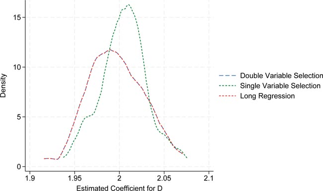
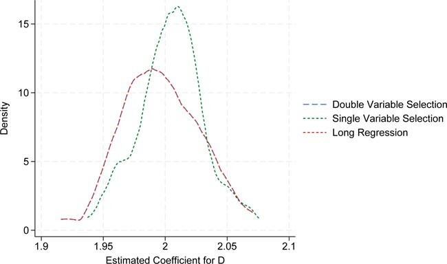
Figure 10 displays the results of a Monte Carlo simulation comparing double and single LASSO feature selection. The experiment is repeated 100 times, with each replication comprising 1000 simulated observations. The red dashed line represents the kernel density estimate for
Monte Carlo simulation for double and single LASSO feature selection. Each replication consists of 1000 simulated observations. The red dashed line represents the kernel estimate of the 100 estimations from the long regression model. The blue dashed line represents the kernel estimate of the 100 regression estimations based on double variable selection. The green dashed line represents the short regression based on single variable selection. Source: Own representation based on simulated datapoints using StataCorp (2023).
Citation: International Food and Agribusiness Management Review 28, 2 (2025) ; 10.22434/ifamr.1087
We observe that the graph for the regression using double variable selection perfectly overlaps with that of the long regression. This indicates that the double variable selection approach successfully eliminates the omitted variable bias that arises with single variable selection when there is a strong correlation between the treatment and the control variable.
Although the example with one control variable is sufficient to illustrate the principle of double selection, incorporating more inputs and different polynomial terms will better reflect real-world applications. In practice, this procedure can be implemented in just two lines of code before proceeding to final estimation with robust standard errors (see Appendix 1 for useful Stata codes). However, it should be emphasized that this method does not protect against issues such as endogenous controls or other specification problems. Nonetheless, this technique shows considerable potential due to its simplicity, which can enhance the robustness of variable selection, as discussed below.
6.2 Discussion of ML variable selection related to p-value mining
There is concern among scientists that some empirical findings cannot be replicated (e.g., Ioannidis, 2005). One factor contributing to this problem may be the treatment of model and variable selection and the subsequent inference (Berk et al., 2013; Leamer, 1983). At the center of the replicability debate is the p-value (Margarian, 2022; Nuzzo, 2014).
The p-value summarizes the incompatibility between a given data set and a proposed model, which typically includes several assumptions such as a null hypothesis that postulates no effect of a variable of interest. The smaller the p-value, the greater the statistical inconsistency between the data and the null hypothesis (Wasserstein et al., 2016). When the p-value falls below an arbitrary threshold (often 0.05), the effect is deemed statistically significant. It is important to stress, however, that although the p-value may be associated with a single estimated coefficient, the statistical test itself is a joint hypothesis asserting both that the effect of the variable of interest is zero and that the model is correctly specified. Therefore, small p-values can be regarded as reliable evidence against the model, including the hypothesis it embodies (Margarian, 2022). Put differently, a small p-value implies rejection of the null hypothesis that the variable of interest has no effect assuming that the model is correctly specified.
Given a correctly specified model, the p-value links the effect size of a variable of interest to its estimation uncertainty, serving as a signal-to-noise ratio. A small p-value indicates that the observed effect is unlikely due to random noise, making it an important statistic when establishing and publishing empirical results. Using a large sample of published papers, Broudeur et al. (2016) find that researchers may inflate the value of just-rejected tests by choosing specifications that yield statistical significance. This practice is often referred to as data mining, p-value mining, HARKing (hypothesizing after the results are known), model fitting, or p-value hacking (e.g. Heckelei et al., 2023). The p-value mining can be viewed as model-selection bias: researchers may choose control variables to maximize rejection of the null rather than to achieve correct specification. The question, then, is which tools can guide variable selection to guard against this bias.
The potential of ML to guide variable selection has been highlighted previously (Urminsky et al., 2016). Variables may be transformed (e.g., raised to the power of 2 or 3) and included as candidates for selection to uncover potential nonlinearities in the controls, a concern that is rarely addressed in applied courses despite the often-unclear degree of nonlinearity. In this context, Hirschauer et al. (2019: p. 719) note that âmodels are regularly populated by differing interaction terms, transformed variables, lagged variables, higher-order polynomials, and control variables. Given the heterogeneity of econometric models, applied economists need consensus regarding the legitimacy and meaning of specification search as well as best practices for replication and meta-analysis.â
Data-driven model selection can help assess the robustness of results, especially given the subjective decisions about variable inclusion and functional forms, because ML model selection is designed to balance model fit with generalizability. Additionally, original studies often cannot be replicated for various reasons (Finger et al., 2023), and ML model selection can provide a range of results across different subsamples to aid replication efforts.
Although these techniques hold promise, they must be treated with caution. For example, Hünermund et al. (2023) stress that there is a risk of including endogenous variables, so-called âbad controlsâ. They demonstrate that double ML is sensitive to even a few such controls, and the resulting bias depends on the theoretical causal model. Furthermore, ML algorithms often involve tuning parameters and other options that can influence the results.
In summary, ML approaches such as LASSO offer a data-driven method to identify which inputs deserve closer attention and may be useful in uncovering unmodeled nonlinearities in various analyses. However, these methods should complement rather than replace thoughtful theoretical consideration (Urminsky et al., 2016).
7. Naive double ML and the FrischâWaughâLovell theorem
This section generalizes the approach from double variable selection to double ML, marking an essential step toward other existing state-of-the-art ML methods. Chernozhukov et al. (2018) outline a more sophisticated estimator compared to double variable selection, that builds on orthogonal moment conditions and crossâfitting. Instead of selecting variables only, the systematic variation between the variables (X and Y; X and D) is removed before estimating the relationship between Y and D, which results in a semiparametric regression as described in Robinson (1988). This framework allows us to integrate a wide range of modern ML methods (such as random forests or deep neural nets) into the estimation process, thereby facilitating valid inference in complex empirical models. This section outlines a naive version to illustrate the overall idea and its relations to the FrischâWaughâLovell theorem (Frisch and Waugh, 1933; Lovell, 1963; Yule, 1907).
The Frisch-Waugh-Lovell theorem is a powerful tool that allows us to reduce multivariate regressions to a series of univariate regressions (Frisch and Waugh, 1933; Lovell, 1963; Yule, 1907). This is especially useful when we are interested in the relationship between two variables while controlling for other factors, which is a common situation in causal inference. The theorem states that when estimating a multivariate regression model of the form,
Y =
the OLS estimator of interest, here  , can be obtained by a two-step procedure:
Step 1: Regress D =  .
.
Step 2: Regress 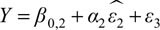 to obtain
  .
.
Because the error term is orthogonal to the variation in X by construction,  represents variation in D net the common variation in D and X and thus . The estimator we are interested in from a multivariate regression can be obtained via a univariate regression. Understanding this principle is extremely useful for grasping how double ML works, as it relies on combining ML-based prediction with orthogonalization. Next, we outline the three essential steps of the double ML procedure.
Step 1: Partial out controls from Y
First, we partial out the variation in Y that correlates with the variation in the controls,
Y = gp(Xâ
) +
Using any ML estimator, we predict Y based on X without the treatment D, i.e.,  and compute the residuals:
Citation: International Food and Agribusiness Management Review 28, 2 (2025) ; 10.22434/ifamr.1087
The residual captures the portion of variation in Y that remains once the variation accounted for by X has been removed.
Step 2: Partial out controls from D
We repeat step one for the variable of interest D:
D = mp(Xâ
) +
We apply any ML algorithm to obtain  .6 We continue and compute the residuals,
Citation: International Food and Agribusiness Management Review 28, 2 (2025) ; 10.22434/ifamr.1087
which captures the variation in D that is orthogonal to X.
Step 3: Estimate the partial effect of D on Y
Finally, we use the residual terms from the previous two steps ( and
and  ):
):
Citation: International Food and Agribusiness Management Review 28, 2 (2025) ; 10.22434/ifamr.1087
The OLS estimate of
7.1 Illustration
A sample of 100 observations is drawn from the following model:
Citation: International Food and Agribusiness Management Review 28, 2 (2025) ; 10.22434/ifamr.1087
Here, the control variable is highly correlated with the treatment, and for illustration purposes, we assign a larger impact on the overall regression. However, experimenting with the correlation between the control and the treatment, adjusting the controlâs influence on the outcome, and adding additional inputs can be very useful.
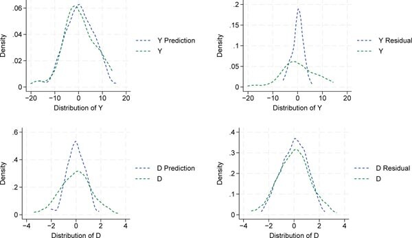
Although any ML method could be used, we continue with the LASSO example. Rather than using LASSO for variable selection, we now use it for prediction. Figure 11 presents the results of the first two steps described in this section.
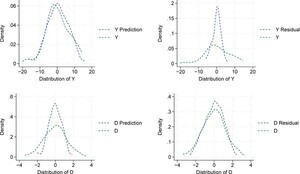
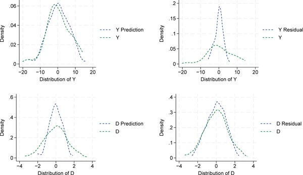
Density functions for predicted and residual variables. The top row shows the outcome variable, and the bottom row shows the treatment variable. In each case, the density of the original variable is depicted in green. On the left, the ML predicted density based on the control variable X is displayed in blue, which is used to partial out the variation due to X. On the right, the blue dashed line represents the density of the residuals after partialling out the variation in X. Own representation based on simulated datapoints using StataCorp (2023).
Citation: International Food and Agribusiness Management Review 28, 2 (2025) ; 10.22434/ifamr.1087
The original densities of the outcome (Y) and the treatment (D) are plotted in green. On the left, the predicted densities based on LASSO feature selection, i.e., and , are plotted in blue. On the right, the residual densities, denoted by and are shown in blue.
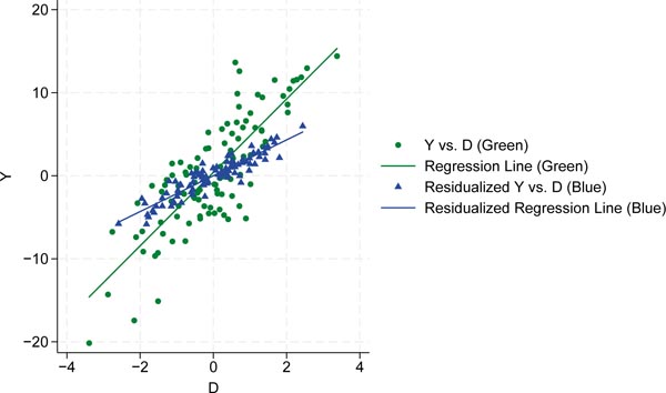
In the final step, we show a scatter plot of the original variables Y and D along with the corresponding regression line in green. In addition, we plot the two residual terms ( and ) and perform the regression. Figure 12 shows the results.
Scatter plots of double residualized variables vs. original variables. the scatter plot of the original variables Y and D, along with the corresponding regression line, is displayed in green. The residual variables, together with their fitted regression line, are shown in blue. Source: Own representation based on simulated datapoints using StataCorp (2023).
Citation: International Food and Agribusiness Management Review 28, 2 (2025) ; 10.22434/ifamr.1087
The residual pairs are depicted as blue triangles, while the original observations appear as green dots. Because the residuals from a regression average zero, the regression line fitted on the residual data must pass through the origin. The slope of this regression line is markedly different from that of the unadjusted model, which fails to account for the variation of X affecting both D and Y.
A key weakness of the naive approach outlined here is that both stages rely on the same dataset. Chernozhukov et al. (2018) address this issue by proposing two variants in which orthogonalization is obtained through cross-fitting, that is, a specific way of applying data splitting. The resulting methods are known as double or debiased ML.
8. Concluding remarks and further reading
This guide demonstrates an accessible and intuitive foundation for grasping modern ML techniques. By employing illustrations with polynomial regressions, key concepts such as the varianceâbias trade-off, overfitting, and regularization can be easily understood. This paper not only clarifies the prediction process but also highlights the adaptations required for causal inference. Since the introduction avoids advanced mathematics, it can be readily integrated into the final two weeks of an undergraduate course.
A variety of textbooks and papers cover the fundamentals of ML. We highly recommend Hastie, Tibshirani, and Friedman (2009) and James et al. (2013). Further, Athey and Imbens (2019) and Storm et al. (2020) provide excellent, accessible overviews of ML techniques. Peters et al. (2017) offer a very detailed exploration of algorithms and their theoretical underpinnings.
As outlined by Chernozhukov et al. (2018), a wide range of modern ML methods such as random forests and deep neural nets can be used for double ML. The algorithms discussed in this paper are available as pre-written commands and packages. For example, several standard packages support double ML in Stata (e.g., dregress, poregress, xpoivregress), in R (Bach et al., 2022), and in Python (Bach et al., 2024).
ML variable selection offers a data-driven approach to identify which inputs deserve closer attention in various analyses, though it should complement rather than replace thoughtful theoretical consideration (Urminsky et al., 2016). For example, causal graphs are important tools in causal inference. They provide a visual framework for encoding assumptions about the causal relationships among variables. These graphs help researchers determine which variables must be controlled to obtain unbiased estimates of causal effects, and they guide both study design and analysis. For further reading on the topic of causal inference, there are a couple of very useful textbooks, e.g., Angrist and Pischke (2009), Chernozhukov et al. (2024), Pearl (2009), Hernán and Robins (2020) and Imbens and Rubin (2015).
One major point to address is the consideration of the resampling procedure. This issue is particularly important in large time series datasets, where temporal dependencies can violate the assumptions underlying standard cross-validation methods. Standard cross-validation may be adapted e.g., fixed-origin cross-validation, rolling-origin cross-validation, or rolling-window cross-validation (Liu and Yang, 2022). Furthermore, when it comes to time series forecasting, the application of cross-validation is not straightforward due to inherent serial correlation and potential non-stationarity. Thus, for time series, so-called blocked cross-validation combined with adequate control for stationarity is important (Bergmeir and BenÃtez, 2012). Nonetheless, standard cross-validation appears to be quite robust compared to time-series-specific techniques (Bergmeir et al., 2018). Generally, the choice of a suitable validation scheme depends on factors such as sample size and becomes even more complex for non-stationarity processes (Schnaubelt, 2019).
Finally, even if ML is not used for model or variable selection, the principle of splitting the sample, distinguishing between training and test data can be valuable for applied researchers and practitioners who select variables manually. For these, it may be useful to split the sample and work with a subset of the data (training data) to identify appropriate methods and model specifications for the problem at hand. Once a specification that works is found, they can proceed to estimate a set of preferred specifications using the full sample, ensuring that the specifications remain unchanged during this transition. Additionally, presenting preliminary results obtained from the training data at conferences can provide valuable input from colleagues on methods and model specifications before moving on to the full sample.
References
Akaike, H. 1973. Maximum likelihood identification of Gaussian autoregressive moving average models. Biometrika 60(2): 255â265.
Angrist, J.D. and J.S. Pischke. 2009. Mostly Harmless Econometrics: An Empiricistâs Companion. Princeton University Press, Princeton, NJ.
Athey, S. and G.W. Imbens. 2019. Machine learning methods that economists should know about. Annual Review of Economics 11(1): 685â725.
Bergmeir, C., R.J. Hyndman and B. Koo. 2018. A note on the validity of cross-validation for evaluating autoregressive time series prediction. Computational Statistics and Data Analysis 120: 70â83.
Bach, P., V. Chernozhukov, M.S. Kurz and M. Spindler. 2022. DoubleML â An object-oriented implementation of double machine learning in Python. Journal of Machine Learning Research 23(53): 1â6. https://www.jmlr.org/papers/v23/21-0862.html.
Bach, P., V. Chernozhukov, M.S. Kurz, M. Spindler and S. Klaassen. 2024. DoubleML â An object-oriented implementation of double machine learning in R. Journal of Statistical Software 108(3): 1â56. https://doi.org/10.18637/jss.v108.i03.
Belloni, A. and V. Chernozhukov 2011. High dimensional sparse econometric models: An introduction. In P. Alguier, E. Gautier and G. Stoltz (Eds), Inverse Problems of High-Dimensional Estimation. Springer, Berlin, pp. 121â156.
Belloni, A., D. Chen, V. Chernozhukov and C.B. Hansen. 2012. Sparse models and methods for optimal instruments with an application to eminent domain. Econometrica 80(6): 2369â2429.
Belloni, A., V. Chernozhukov and C. Hansen. 2014a. Inference on treatment effects after selection among high-dimensional controls. The Review of Economic Studies 81(2): 608â650.
Belloni, A., V. Chernozhukov and C. Hansen. 2014b. High-dimensional methods and inference on structural and treatment effects. Journal of Economic Perspectives 28(2): 29â50.
Bergmeir, C. and J.M. BenÃtez. 2012. On the use of crossâvalidation for time series predictor evaluation. Information Sciences 191: 192â213.
Berk, R., L. Brown, A. Buja, K. Zhang and L. Zhao. 2013. Valid post-selection inference. The Annals of Statistics 41(2): 802â837.
Breiman, L. 2001. Statistical modeling: The two cultures (with comments and a rejoinder by the author. Statistical Science 16(3): 199â231.
Breiman, L. and P. Spector. 1992. Submodel selection and evaluation in regression. The X-random case. International Statistical Review 60(3): 291â319.
Brodeur, A., M. Lé, M. Sangnier and Y. Zylberberg. 2016. Star wars: The empirics strike back. American Economic Journal: Applied Economics 8(1): 1â32.
Bühlmann, P. and S. Van De Geer. 2011. Statistics for high-dimensional data: methods, theory and applications. Springer, Berlin.
Chernozhukov, V., C. Hansen, N. Kallus, M. Spindler and V. Syrgkanis. 2024. Applied causal inference powered by ML and AI. Available online at https://causalml-book.org; arXiv:2403.02467.
Chernozhukov, V., D. Chetverikov, M. Demirer, E. Duflo, C. Hansen, W. Newey and J. Robins. 2018. Double/debiased machine learning for treatment and structural parameters. The Econometrics Journal 21(1): C1âC68.
Chetverikov, D., Z. Liao and V. Chernozhukov. 2021. On cross-validated lasso in high dimensions. The Annals of Statistics 49(3): 1300â1317.
Cunningham, S. 2021. Causal inference: The mixtape. Yale University Press, London.
Dudoit, S. and J.J. Van Der Laan. 2005. Asymptotics of cross-validated risk estimation in estimator selection and performance assessment. Statistical Methodology 2(2): 131â154.
Dunning, T. 2010. Design-based inference: Beyond the pitfalls of regression analysis? In D. Collier and H.E. Brady (Eds), Rethinking Social Inquiry: Diverse Tools, Shared Standards. Rowman & Littlefield, London, pp. 273â311.
Dumelle, M., M. Higham, J.M. Verhoef, A.R. Olsen and L. Madsen. 2022. A comparison of designâbased and modelâbased approaches for finite population spatial sampling and inference. Methods in Ecology and Evolution 13(9): 2018â2029.
Efron, B. and C. Morris. 1975. Data analysis using Steinâs estimator and its generalizations. Journal of the American Statistical Association 70(350): 311â319.
Efron, B. and C. Morris. 1977. Steinâs paradox in statistics. Scientific American 236(5): 119â127.
Funk, M.J., D. Westreich, C. Wiesen, T. Stürmer, M.A. Brookhart and M. Davidian. 2011. Doubly robust estimation of causal effects. American Journal of Epidemiology 173(7): 761â767.
Farebrother, R.W. 1976. Further results on the mean square error of ridge regression. Journal of the Royal Statistical Society, Series B (Methodological) 38: 248â250.
Fisher, R.A. 1922. On the mathematical foundations of theoretical statistics. Philosophical transactions of the Royal Society of London. Series A, containing papers of a mathematical or physical character 222(594â604): 309â368.
Finger, R., C. Grebitus and A. Henningsen. 2023. Replications in agricultural economics. Applied Economic Perspectives and Policy 45(3): 1258â1274.
Frisch, R. and F.V. Waugh. 1933. Partial time regressions as compared with individual trends. Econometrica: Journal of the Econometric Society 1(4): 387â401.
Fricker Jr., R.D., K. Burke, X. Han and W.H. Woodall. 2019. Assessing the statistical analyses used in basic and applied social psychology after their p-value ban. The American Statistician 73(Suppl. 1): 374â384.
Gelman, A., J.B. Carlin, H.S. Stern, D.B. Dunson, A. Vehtari and D.B. Rubin. 2013. Bayesian Data Analysis, 3rd edn. Chapman and Hall/CRC, Boca Raton, FL.
Golub, G.H., M. Heath and G. Wahba. 1979. Generalized cross-validation as a method for choosing a good ridge parameter. Technometrics 21(2): 215â223.
Hastie, T., R. Tibshirani and J.H. Friedman. 2009. The elements of statistical learning: data mining, inference, and prediction, 2nd edn. Springer, New York, NY.
Hawkins, D.M. 2004. The problem of overfitting. Journal of Chemical Information and Computer Sciences 44(1): 1â12.
Heckelei, T., S. Hüttel, M. Odening and J. Rommel. 2023. The p-value debate and statistical (mal)practiceâImplications for the agricultural and food economics community. German Journal of Agricultural Economics 72(1): 47â67.
Hernán, M.A. and J.M. Robins. 2020. Causal inference: what if. Chapman and Hall/CRC, Boca Raton, FL.
Hirschauer, N., S. Grüner, O. MuÃhoff and C. Becker. 2019. Twenty steps towards an adequate inferential interpretation of p-values in econometrics. Jahrbücher für Nationalökonomie und Statistik 239(4): 703â721.
Holland, P.W. 1986. Statistics and causal inference. Journal of the American Statistical Association 81(396): 945â960.
Hünermund, P., B. Louw and I. Caspi. 2023. Double machine learning and automated confounder selection: A cautionary tale. Journal of Causal Inference 11(1): 20220078.
Imbens, G.W. 2021. Statistical significance, p-values, and the reporting of uncertainty. Journal of Economic Perspectives 35(3): 157â174.
Imbens, G.W. and D.B. Rubin. 2015. Causal inference in statistics, social, and biomedical sciences. Cambridge University Press, Cambridge.
Imbens, G.W. and J.M. Wooldridge. 2009. Recent developments in the econometrics of program evaluation. Journal of Economic Literature 47(1): 5â86.
Ioannidis, J.P. 2005. Why most published research findings are false. PLoS Medicine 2(8): e124.
James, G., D. Witten, T. Hastie and R. Tibshirani. 2013. An introduction to statistical learning. With applications in R. Springer, New York, NY.
Leeb, H. and B.M. Pötscher. 2006. Can one estimate the conditional distribution of post-model-selection estimators? The Annals of Statistics 34(5): 2554â2591.
Leamer, E.E. 1983. Letâs take the con out of econometrics. The American Economic Review 73(1): 31â43.
Liu, Z. and X. Yang. 2022. Cross validation for uncertain autoregressive model. Communications in Statistics-Simulation and Computation 51(8): 4715â4726.
Lovell, M.C. 1963. Seasonal adjustment of economic time series and multiple regression analysis. Journal of the American Statistical Association 58(304): 993â1010.
Margarian, A. 2022. Beyond p-value-obsession: When are statistical hypothesis tests required and appropriate? German Journal of Agricultural Economics 71(4): 213â226.
Mittelhammer, R.C. 2002. Mathematical Statistics for Economics and Business. Springer, New York, NY.
McCullagh, P. 2002. What is a statistical model? The Annals of Statistics 30(5): 1225â1310.
Neyman, J. 1934. On the two different aspects of the representative method: The method of stratified sampling and the method of purposive selection. Journal of the Royal Statistical Society 97(4): 558â625.
Nuzzo, R. 2014. Statistical errors. Nature 506(7487): 150.
Paluck, E.L. and D.P. Green. 2009. Prejudice reduction: what works? A review and assessment of research and practice. Annual Review of Psychology 60: 339â367.
Pearl, J. 2009. Causality. Cambridge University Press, Cambridge.
Pesaran, M.H. 2015. Time Series and Panel Data Econometrics. Oxford University Press, Oxford.
Peters, J., D. Janzing and B. Schölkopf. 2017. Elements of causal inference: foundations and learning algorithms. The MIT Press, Cambridge, MA.
Rosenbaum, P.R. and D.B. Rubin. 1983. The central role of the propensity score in observational studies for causal effects. Biometrika 70(1): 41â55.
Robins, J., M. Sued, Q. Lei-Gomez and A. Rotnitzky. 2007. Comment: Performance of double-robust estimators when âinverse probabilityâ weights are highly variable. Statistical Science 22(4): 544â559.
Robinson, P.M. 1988. Root-N-consistent semiparametric regression. Econometrica 56(4): 931â954.
Rubin, D.B. 1990. Comment: Neyman (1923) and causal inference in experiments and observational studies. Statistical Science 5(4): 472â480.
Schnaubelt, M. 2019. A comparison of machine learning model validation schemes for non-stationary time series data. FAU Discussion Papers in Economics 11/2019. Institute for Economics, Friedrich-Alexander-Universität Erlangen-Nürnberg, Nuremberg.
StataCorp 2023. Stata Statistical Software, Release 18. StataCorp, College Station, TX.
Schwarz, G. 1978. Estimating the dimension of a model. The Annals of Statistics 6(2): 461â464.
Shao, J. 1993. Linear model selection by cross-validation. Journal of the American Statistical Association 88(422): 486â494.
Steegen, S., S. Tuerlinck, A. Gelman and W. Vanpaemel. 2016. Increasing transparency through a multiverse analysis. Perspectives on Psychological Science 11(5): 702â712.
Sterba, S.K. 2009. Alternative model-based and design-based frameworks for inference from samples to populations: from polarization to integration. Multivariate Behavioral Research 44(6): 711â740.
Stone, M. 1977. An asymptotic equivalence of choice of model by crossâvalidation and Akaikeâs criterion. Journal of the Royal Statistical Society: Series B (Methodological) 39(1): 44â47.
Storm, H., K. Baylis and T. Heckelei. 2020. Machine learning in agricultural and applied economics. European Review of Agricultural Economics 47(3): 849â892.
Taboga, M. 2021. Ridge regression. Lectures on Probability Theory and Mathematical Statistics. Available online at https://www.statlect.com/fundamentals-of-statistics/ridge-regression.
Theobald, C.M. 1974. Generalizations of mean square error applied to ridge regression. Journal of the Royal Statistical Society, Series B (Methodological) 36: 103â106.
Urminsky, O., C. Hansen and V. Chernozhukov. 2016. Using double-LASSO regression for principled variable selection. Available online at https://home.uchicago.edu/ourminsky/Variable_Selection.pdf.
Wasserstein, R.L. and N.A. Lazar. 2016. The ASA statement on p-values: Context, process, and purpose. The American Statistician 70(2): 129â133.
Wooldridge, J.M. 2015. Introductory Econometrics: A Modern Approach. Cengage Learning, London.
Yule, G.U. 1907. On the theory of correlation for any number of variables, treated by a new system of notation. Proceedings of the Royal Society of London, Series A 79(529): 182â193.
Zou, H. and T. Hastie. 2005. Regularization and variable selection via the elastic net. Journal of the Royal Statistical Society: Series B (Statistical Methodology) 67(2): 301â320.
Appendix 1: Simple Stata Codes
/*Step1*/ lasso linear Y x1, selection(cv)
/*Step2*/ lasso linear D x1, selection(cv)
/*Step3*/ regress Y D /*Selected variables from step 1 and 2*/, robust
/*Double variable selection Step1-Step3*/ dsregress Y D, controls(x1) selection(cv)
/*Double partialling out*/ poregress Y D, controls(x1) selection(cv)
/*Cross-fit double partialling out*/ xporegress Y D, controls(x1) selection(cv)
Appendix 2
(A1) Y =
(A2) D = mp(Xâ
) +
Substitute selection error:
(A3.1)Y =
(A3.2) Y =
Define:
rc = (rY +
gp(Xâ ) = g(Xâ ) +rc
g(Xâ
) =
Substitute definitions:
(A4) Y = gp(Xâ
) +
See, for example, Hastie et al. (2009: Chapter 2), where this expression is evaluated at a specific point. In general, the unconditional MSE provides a global measure of prediction error, while the conditional MSE quantifies the error at a specific input value.
For a more robust version of the LASSO, see the elastic net (Zou and Hastie, 2005).
Useful tools in this context are Directed Acyclic Graphs (DAGs), which offer a visual map that facilitates critical and transparent reflection on causal assumptions (e.g., Chernozhukov et al., 2024).
The expected value can also be conditioned on X, which gives the conditional average treatment effect (CATE). Instead of assuming a constant treatment effect (
See, for example, Chetverikov et al. (2021). Other approaches include adaptive LASSO and plugâin estimators with different sparsity constraints (Belloni and Chernozhukov, 2011; Belloni et al., 2014; Bühlmann and van de Geer, 2011).
Note the similarities to the instrumental variable estimator. If D is suspected to be endogenous and X represents a set of exogenous potential instruments, then the ML estimate can serve as an optimal instrument. For further discussion, please refer to Belloni et al. (2012).


